The GARCH-DCC Model and 2-stage DCC(MVT) estimation.

This short demonstration illustrates the use of the DCC model and its methods using the rmgarch package, and in particular an alternative method for 2-stage DCC estimation in the presence of the MVT distribution shape (nuisance) parameter. The theoretical background and representation of the model is detailed in the package’s vignette. The dataset and period used are purely for illustration purposes.

library(rmgarch)
library(parallel)
data(dji30retw)
Dat = dji30retw[, 1:10, drop = FALSE]
# define a DCCspec object: 2 stage estimation should usually always use
# Normal for 1-stage (see below for
xspec = ugarchspec(mean.model = list(armaOrder = c(1, 1)), variance.model = list(garchOrder = c(1,1), model = 'eGARCH'), distribution.model = 'norm')
uspec = multispec(replicate(10, xspec))
spec1 = dccspec(uspec = uspec, dccOrder = c(1, 1), distribution = 'mvnorm')
spec1a = dccspec(uspec = uspec, dccOrder = c(1, 1), model='aDCC', distribution = 'mvnorm')
spec2 = dccspec(uspec = uspec, dccOrder = c(1, 1), distribution = 'mvlaplace')
spec2a = dccspec(uspec = uspec, dccOrder = c(1, 1), model='aDCC', distribution = 'mvlaplace')

Since multiple DCC models are being estimated on the same dataset with the same first stage dynamics, we can estimate the first stage once and pass it to the dccfit routine (rather than re-estimating it every time dccfit is called):

cl = makePSOCKcluster(10)
multf = multifit(uspec, Dat, cluster = cl)

Next, the second stage of the DCC model is estimated.

fit1 = dccfit(spec1, data = Dat, fit.control = list(eval.se = TRUE), fit = multf, cluster = cl)
fit1a = dccfit(spec1a, data = Dat, fit.control = list(eval.se = TRUE), fit = multf, cluster = cl)
fit2 = dccfit(spec2, data = Dat, fit.control = list(eval.se = TRUE), fit = multf, cluster = cl)
fit2a = dccfit(spec2a, data = Dat, fit.control = list(eval.se = TRUE), fit = multf, cluster = cl)

To fit the DCC (MVT) model in practice, one either assumes a first stage QML, else must jointly estimate in 1 stage the common shape parameter. In the example that follows below, an alternative approach is used to approximate the common shape parameter.

# First Estimate a QML first stage model (multf already estimated). Then
# estimate the second stage shape parameter.
spec3 = dccspec(uspec = uspec, dccOrder = c(1, 1), distribution = 'mvt')
fit3 = dccfit(spec3, data = Dat, fit.control = list(eval.se = FALSE), fit = multf)
# obtain the multivariate shape parameter:
mvt.shape = rshape(fit3)
# Plug that into a fixed first stage model and iterate :
mvt.l = rep(0, 6)
mvt.s = rep(0, 6)
mvt.l[1] = likelihood(fit3)
mvt.s[1] = mvt.shape
for (i in 1:5) {
xspec = ugarchspec(mean.model = list(armaOrder = c(1, 1)), variance.model = list(garchOrder = c(1,1), model = 'eGARCH'), distribution.model = 'std', fixed.pars = list(shape = mvt.shape))
spec3 = dccspec(uspec = multispec(replicate(10, xspec)), dccOrder = c(1,1), distribution = 'mvt')
fit3 = dccfit(spec3, data = Dat, solver = 'solnp', fit.control = list(eval.se = FALSE))
mvt.shape = rshape(fit3)
mvt.l[i + 1] = likelihood(fit3)
mvt.s[i + 1] = mvt.shape
}
# Finally, once more, fixing the second stage shape parameter, and
# evaluating the standard errors
xspec = ugarchspec(mean.model = list(armaOrder = c(1, 1)), variance.model = list(garchOrder = c(1,1), model = 'eGARCH'), distribution.model = 'std', fixed.pars = list(shape = mvt.shape))
spec3 = dccspec(uspec = multispec(replicate(10, xspec)), dccOrder = c(1, 1), distribution = 'mvt', fixed.pars = list(shape = mvt.shape))
fit3 = dccfit(spec3, data = Dat, solver = 'solnp', fit.control = list(eval.se = TRUE), cluster = cl)

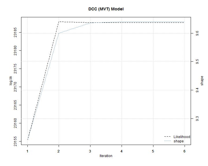
The plot in the change of the likelihood and shape shows that only a few iterations are necessary to converge to a stable value.
dccmvt_1

The value of the shape parameter implies an excess kurtosis of 1.06. The exercise is repeated for the asymmetric DCC (MVT) model.

xspec = ugarchspec(mean.model = list(armaOrder = c(1,1)), variance.model = list(garchOrder = c(1,1), model = "eGARCH"),  distribution.model = "norm")
spec3a  = dccspec(uspec = multispec( replicate(10, xspec) ), dccOrder = c(1,1), distribution = "mvt", model="aDCC")
fit3a = dccfit(spec3a, data = Dat, fit.control = list(eval.se=FALSE), fit = multf)
# obtain the multivariate shape parameter:
mvtx.shape = rshape(fit3a)
# Plug that into a fixed first stage model and iterate :
mvtx.l = rep(0, 6)
mvtx.s = rep(0, 6)
mvtx.l[1] = likelihood(fit3)
mvtx.s[1] = mvtx.shape
for(i in 1:5){
xspec = ugarchspec(mean.model = list(armaOrder = c(1,1)), variance.model = list(garchOrder = c(1,1), model = "eGARCH"),  distribution.model = "std", fixed.pars = list(shape=mvtx.shape))
spec3a = dccspec(uspec = multispec( replicate(10, xspec) ), dccOrder = c(1,1), model="aDCC", distribution = "mvt")
fit3a = dccfit(spec3a, data = Dat, solver = "solnp", fit.control = list(eval.se=FALSE))
mvtx.shape = rshape(fit3a)
mvtx.l[i+1] = likelihood(fit3a)
mvtx.s[i+1] = mvtx.shape
}
# Finally, once more, fixing the second stage shaoe parameter, and evaluating the standard errors
xspec = ugarchspec(mean.model = list(armaOrder = c(1,1)), variance.model = list(garchOrder = c(1,1), model = "eGARCH"),  distribution.model = "std", fixed.pars = list(shape=mvtx.shape))
spec3a = dccspec(uspec = multispec( replicate(10, xspec) ), dccOrder = c(1,1), model="aDCC", distribution = "mvt", fixed.pars=list(shape=mvtx.shape))
fit3a = dccfit(spec3a, data = Dat, solver = "solnp", fit.control = list(eval.se=TRUE), cluster = cl)

The table below displays the summary of the estimated models, where the stars next to the coefficients indicate the level of significance (*** 1%, ** 5%, * 10%). The asymmetry parameter is everywhere insignificant and, not surprisingly, the MVT distribution provides for the best overall fit (even when accounting for one extra parameter estimated).

##           DCC-MVN   aDCC-MVN    DCC-MVL   aDCC-MVL      DCC-MVT     aDCC-MVT
## a      0.00784*** 0.00639*** 0.00618***  0.0055***   0.00665***    0.00623***
## b      0.97119*** 0.96956*** 0.97624*** 0.97468***   0.97841***    0.97784***
## g                    0.00439               0.00237                 0.00134
## shape                                                9.63947***    9.72587***
## LogLik      22812      22814      22858      22859        23188         23188

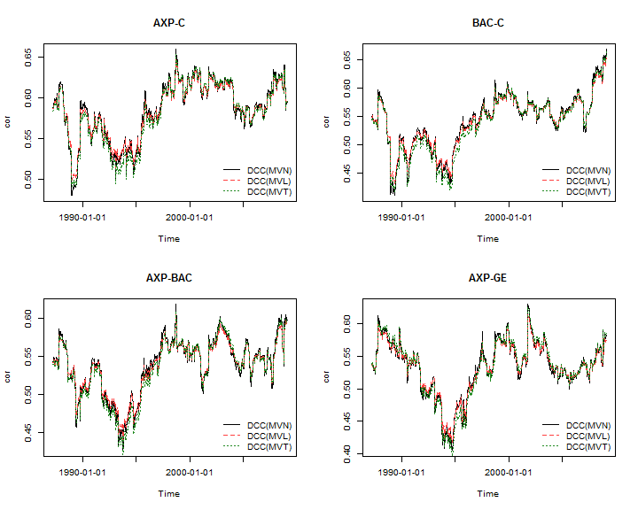
To complete the demonstration, the plots below illustrate some of the dynamic correlations from the different models:
dccmvt_2


…and remember to terminate the cluster object:

stopCluster(cl)
Rolling GARCH Forecasts

The rugarch package contains a rolling volatility forecast function called ugarchroll, but in this example I will show how easy it is to create a quick custom function. Having a rolling forecast of volatility can prove an invaluable indicator for use in trading systems. an example of which is also included.

# The function makes exclusive use of xts based timeseries indexing.
garchv = function(x, start = 600, roll = 25, n.ahead = 1, spec = NULL, cluster = NULL)
{
# x : is a series of closing prices

# start : is the number of periods which are used for the first rolling
# estimation window

# roll : the number of periods to roll the 1-ahead forecast before
# re-estimating the model parameters

# n.ahead : the forecast horizon

# spec : the univariate GARCH model specification (uGARCHspec object)

# cluster : a pre-created cluster object from the parallel package
require(rugarch)
if (!is.xts(x))
stop('\nx must be an xts object')
# create continuous return series
r = na.omit(diff(log(x), 1))
n = nrow(r)
if (n <= start)
stop('\nstart cannot be greater than length of x')
# the ending points of the estimation window
s = seq(start + roll, n, by = roll)
m = length(s)
# the rolling forecast length
out.sample = rep(roll, m)
# adjustment to include all the datapoints from the end
if (s[m] < n) {
s = c(s, n)
m = length(s)
out.sample = c(out.sample, s[m] - s[m - 1])
}
# the default specification if none is provided is set to an eGARCH-std
# model
if (is.null(spec))
spec = ugarchspec(variance.model = list(model = 'eGARCH'), distribution = 'std')
if (!is.null(cluster)) {
clusterEvalQ(cluster, library(rugarch))
clusterEvalQ(cluster, library(xts))
clusterExport(cluster, varlist = c('r', 's', 'roll', 'spec', 'out.sample'),
envir = environment())
tmp = clusterApply(cl = cluster, 1:m, fun = function(i) {
fit = ugarchfit(spec, r[1:s[i], ], out.sample = out.sample[i], solver = 'hybrid')
f = ugarchforecast(fit, n.ahead = 1, n.roll = out.sample[i] - 1)
y = sigma(f)
# use xts for indexing the forecasts
y = xts(as.numeric(y), tail(time(r[1:s[i], ]), out.sample[i]))
return(y)
})
} else{
tmp = lapply(1:m, FUN = function(i) {
fit = ugarchfit(spec, r[1:s[i], ], out.sample = out.sample[i], solver = 'hybrid')
f = ugarchforecast(fit, n.ahead = 1, n.roll = out.sample[i] - 1)
y = sigma(f)
# use xts for indexing the forecasts
y = xts(as.numeric(y), tail(time(r[1:s[i], ]), out.sample[i]))
return(y)
})
}
# re-assemble the forecasts
forc = tmp[[1]]
for (i in 2:m) {
forc = rbind(forc, tmp[[i]])
}
colnames(forc) = 'V'
return(forc)
}

As an application of a rolling volatility forecast, I will consider the variable moving average (VMA) indicator of Chande (see Technical Analysis of Stocks & Commodities, March 1992), implemented in the TTR package.

getSymbols('SPY', src = 'yahoo', from = '1990-01-01')
SPY = adjustOHLC(SPY, use.Adjusted = TRUE)
library(parallel)
cluster = makePSOCKcluster(10)
garch_V = garchv(Cl(SPY), start = 600, roll = 25, n.ahead = 1, spec = NULL,
cluster = cluster)
stopCluster(cluster)

The VMA function uses a weighting vector, scaled between 0 and 1, with higher values (volatility) leading to faster adjustment of the moving average. Formally, it is defined as $$VM{A_t} = \left( {r{w_t}} \right){P_t} + \left( {1 – r{w_t}} \right)VM{A_{t – 1}}$$ where r is the decay ratio which adjusts the smoothness of the moving average, and w the weighting vector. In order to use the forecast volatility with the VMA indicator we need to rescale it to lie between the required bounds. A simple transformation which uses the min and max values can be used, such that $\bar h=\left(max(h)-h\right)/\left(\max(h)-min(h)\right)$. A slight problem with this approach is that the max and min of the forecast for the period is not known (not without looking ahead), but we ignore this problem at present.

barh = (garch_V - min(garch_V))/(max(garch_V) - min(garch_V))
tmp = cbind(Cl(SPY), barh)
tmp = na.omit(tmp)
VMA_garch1 = VMA(tmp[, 1], w = tmp[, 2]^2, ratio = 0.1)
VMA_garch2 = VMA(tmp[, 1], w = tmp[, 2]^2, ratio = 1)

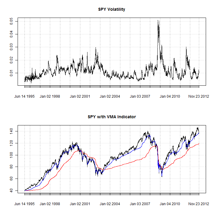
For illustration, I’ll plot 2 VMA, a slow and fast version, the calibration of which is done through the decay ‘ratio’ option in the VMA function.

par(mfrow = c(2, 1))
plot(garch_V, main = 'SPY Volatility')
plot(tmp[, 1], main = 'SPY w/th VMA Indicator')
lines(VMA_garch1, col = 2)
lines(VMA_garch2, col = 4)

rolling_var_1

As can be visually inferred, the effect of the spikes in volatility on the moving average indicator are clearly illustrated, particularly around the 2008 period. A simple system would probably seek to be long the security when the fast moving average is above the slow moving average, when markets are trending.

How Good Are Your VaR Estimates?

Despite its shortcomings, Value at Risk (VaR) is still the most widely used measure for measuring the risk of a portfolio, and the preferred measure in the Basel II Accord. In this demonstration, I backtest a group of indices using a GARCH-DCC(MVT) model and test the VaR obtained from randomly weighted portfolio margins using a number of relevant tests, based on functions in the rugarch and rmgarch packages. The use of randomly generated weights is in order to avoid any bias from testing a model with only equal weighted margins which is sometimes used. In practise, the weight vector is pre-determined, but for the backtesting, this approach appears a reasonable compromise for evaluating multivariate models using only univariate measures.

library(rmgarch)
library(quantmod)
# International Equity ETFs
Symbols = c('SPY', 'EWC', 'EWW', 'EWA', 'EWH', 'EWJ', 'EWS', 'EWG',
'EWQ', 'EWP', 'EWI', 'EWU', 'EWL', 'EWD')
m = length(Symbols)
Countries = c('USA', 'Canada', 'Mexico', 'Australia', 'Hong.Kong',
'Japan', 'Singapore', 'Germany', 'France', 'Spain', 'Italy', 'UK',
'Switzerland', 'Sweden')
getSymbols(Symbols, src = 'yahoo', from = '1990-01-01')
Y = Ad(SPY)
for (i in 2:m) Y = cbind(R, Ad(get(Symbols[i])))
Y = na.omit(Y)
R = ROC(Y, na.pad = FALSE)

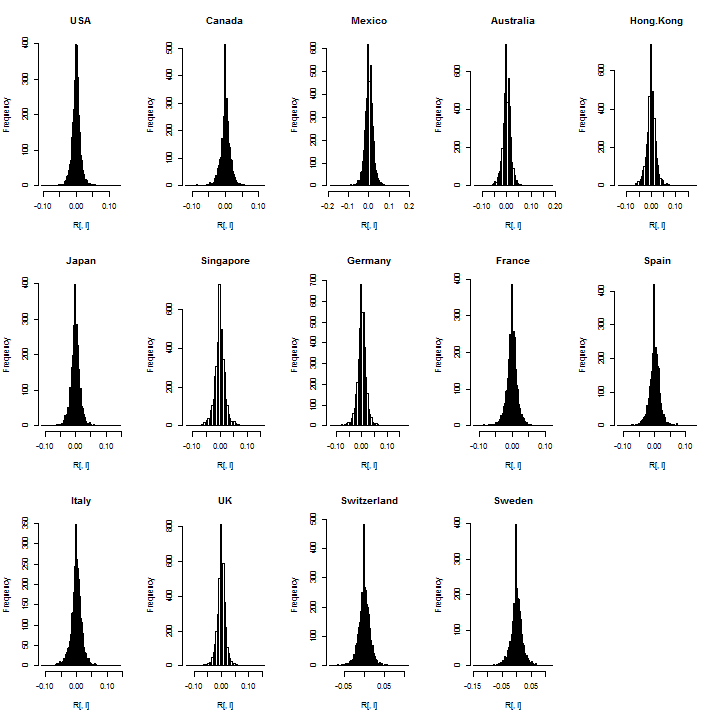
It’s always a good idea to check the data visually for outliers or bad data:

par(mfrow = c(3, 5))
for (i in 1:m) hist(R[, i], breaks = 100, main = Countries[i])

var_estimates_1

Not suprisingly, there is a large spike for the zeros in many countries and this is likely related to low volume when these ETFs where first introduced in the mid 1990s. I’ll exclude about 100 days from the start, since consecutive zeros in a dataset can seriously affect estimation (particularly a rolling backtest which does not use all the sample at once).

R = R[-c(1:100), ]

This is a ‘large’ scale backtest, so full use of parallel functionality is made, which is one of the features of the multivariate GARCH models included in the rmgarch package (the separability of the univariate from the multivariate dynamics).
A 2-stage QML DCC-(MVT) model (with first stage based ARMA(1,1)-gjrGARCH dynamics) is adopted, in the same spirit as in Bauwens and Laurent (2005). A separate post provides for an alternative approach using an iterated procedure for joint shape parameter estimation in the first stage conditional student density.
The model is estimated every 25 days (approx. 1 month), using all the data available up to that point, and the rolling 1-ahead forecast for the next 25 days is evaluated. The backtest procedure starts on 02-06-1999, thus providing an initial window for estimation of size 800, and ends on 10-19-2012 (the code adjusts to the last date available from the downloaded data.)

n = nrow(R)
roll = 25
start = 800
s = seq(start + roll, n, by = roll)
p = length(s)
out.sample = rep(roll, p)
if (s[p] < n) {
out.sample = c(out.sample, n - s[p])
s = c(s, n)
p = length(s)
}

500 sets of random weights (no shorts) are generated with full investment constraint (and for replicability the random seed is initialized to a predefined integer).

set.seed(111111)
w = matrix(rexp(14 * 500), 500, 14)
w = t(apply(w, 1, FUN = function(x) x/sum(x)))
w[500, ] = rep(1/m, m)
# create a required function for use later.
wsig = function(s, w) apply(w, 1, FUN = function(x) sqrt(x %*% s %*% x))

The backtest returns a list of length sum(out.sample)=3288 with elements the 25-rolling 1-ahead conditional forecasts of the mean and sigma weighted by the 500 random weight sets, and a vector of the shape parameter for each forecast window. While 2-stage DCC models offer the possibility of large scale parallel estimation because of the separation of the univariate and multivariate likelihoods, the calculation of the partitioned standard error (s.e.) matrix is quite slow (though this too can take advantage of parallel methods). For this application, s.e. are not calculated.

# set up the parallel estimation
library(parallel)
spec = multispec(replicate(m, ugarchspec(variance.model = list(model
= 'gjrGARCH'))))
mspec = dccspec(spec, distribution = 'mvt')
cl < - makePSOCKcluster(20)
clusterEvalQ(cl = cl, library(rmgarch))
clusterEvalQ(cl = cl, library(xts))
clusterExport(cl, varlist = c('R', 's', 'w', 'mspec', 'wsig', 'out.sample'),
envir = environment())
tic = Sys.time()
mod = clusterApply(cl = cl, 1:p, fun = function(i) {
fit = dccfit(mspec, R[1:s[i], ], out.sample = out.sample[i],
solver = 'solnp', fit.control = list(eval.se = FALSE))
f = dccforecast(fit, n.ahead = 1, n.roll = out.sample[i] - 1)
mu = t(apply(f@mforecast$mu, 3, FUN = function(x) x))
mu = apply(w, 1, FUN = function(x) mu %*% x)
# rcov(DCCforecast) is a list of size n.roll+1, with each
# element being an array of size m by m by n.ahead
sig = t(sapply(rcov(f), FUN = function(x) wsig(x[, , 1], w)))
shape = rep(as.numeric(rshape(fit)), out.sample[i])
dt = as.character(tail(time(R[1:s[i], ]), out.sample[i]))
ans = list(mu = mu, sig = sig, shape = shape, dates = dt)
return(ans)
})
toc = Sys.time()
stopCluster(cl)

The total time taken is about 3.62 mins, but with cloud based computing this could certainly be reduced, given that the functions themselves can take advantage of parallel estimation (not used here) to estimate the univariate models. Next, the forecasts are  re-assembled and the VaR calculated, which because of the location and scaling invariant property of this distribution, is quite fast to evaluate.

mu = sig = shape = Dates = NULL
for (i in 1:length(mod)) {
mu = rbind(mu, mod[[i]]$mu)
sig = rbind(sig, mod[[i]]$sig)
shape = c(shape, mod[[i]]$shape)
Dates = c(Dates, mod[[i]]$dates)
}
# The realized weighted returns
realized = apply(w, 1, FUN = function(x) tail(R, sum(out.sample)) %*% x)
VaR01 = VaR05 = matrix(NA, ncol = 500, nrow = sum(out.sample))
for (i in 1:500) {
VaR01[, i] = mu[, i] + sig[, i] * qdist('std', 0.01, mu = 0, sigma = 1,
shape = shape)
VaR05[, i] = mu[, i] + sig[, i] * qdist('std', 0.05, mu = 0, sigma = 1,
shape = shape)
}

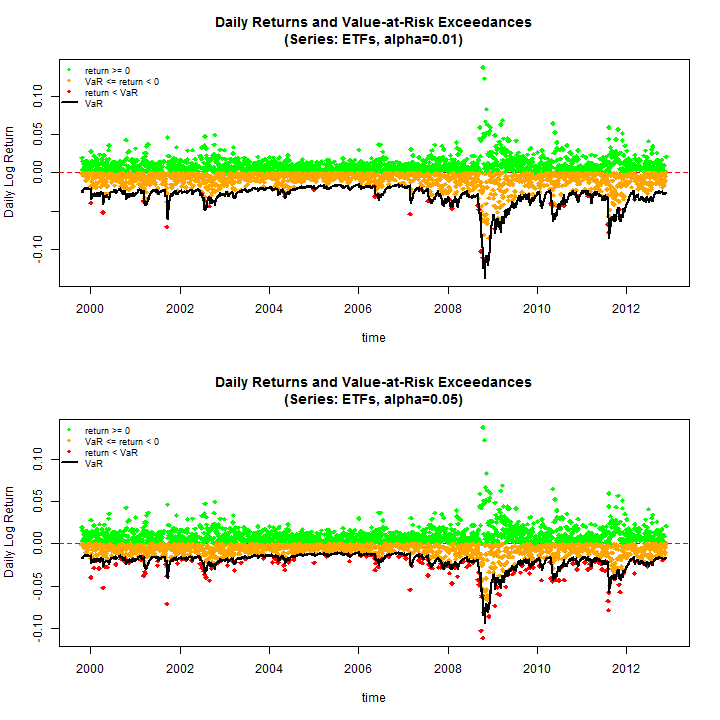
Before proceeding to the tests, do some plots to see some of the results (use the equal weighting margin=500)

par(mfrow = c(2, 1))
rugarch:::.VaRplot('ETFs', 0.01, realized[, 500], Dates, VaR01[, 500])
rugarch:::.VaRplot('ETFs', 0.05, realized[, 500], Dates, VaR05[, 500])

var_estimates_2

The test of VaR exceedances and VaR Duration are used, both of which are implemented and described in detail in the rugarch vignette and documentation. Once again, parallel functionality is used to evaluate these tests. For the exceedances test only the conditional coverage test is considered.

f = function(VaR, realized, p) {
tmp1 = VaRTest(p, realized, VaR)
tmp2 = VaRDurTest(p, realized, VaR)
Exceed = tmp1$actual.exceed
Excp = tmp1$cc.LRp
Excs = tmp1$cc.LRstat
Durb = tmp2$b
Durp = tmp2$LRp
return(c(Exceed = Exceed, Excp = Excp, Excs = Excs, Durb = Durb, Durp = Durp))
}
cl < - makeCluster(20)
clusterEvalQ(cl = cl, library(rugarch))
clusterExport(cl, varlist = c('VaR01', 'VaR05', 'f', 'realized'), envir = environment())
test1pct = clusterApply(cl = cl, 1:500, fun = function(i) f(VaR01[, i], realized[,
i], 0.01))
test5pct = clusterApply(cl = cl, 1:500, fun = function(i) f(VaR05[, i], realized[,
i], 0.05))
stopCluster(cl)
test1pct = t(sapply(test1pct, FUN = function(x) x))
test5pct = t(sapply(test5pct, FUN = function(x) x))
VaRresults = matrix(NA, ncol = 2, nrow = 5)
VaRDurresults = matrix(NA, ncol = 2, nrow = 3)
rownames(VaRDurresults) = c('Median_[b]', 'Median_pvalue', '%Rejections')
rownames(VaRresults) = c('Mean_Exceedances', 'E[Exceedances]', 'Median_stat',
'Median_pvalue', '%Rejections')
colnames(VaRDurresults) = colnames(VaRresults) = c('VaR[1%]', 'VaR[5%]')
VaRresults[1, ] = c(mean(test1pct[, 1]), mean(test5pct[, 1]))
VaRresults[2, ] = c(floor(sum(out.sample) * 0.01), floor(sum(out.sample) * 0.05))
VaRresults[3, ] = c(mean(test1pct[, 3]), median(test5pct[, 3]))
VaRresults[4, ] = c(mean(test1pct[, 2]), median(test5pct[, 2]))
VaRresults[5, ] = c(100 * length(which(test1pct[, 2] < 0.05))/nrow(test1pct),
100 * length(which(test5pct[, 2] < 0.05))/nrow(test5pct))
VaRDurresults[1, ] = c(median(test1pct[, 4]), median(test5pct[, 4]))
VaRDurresults[2, ] = c(median(test1pct[, 5]), median(test5pct[, 5]))
VaRDurresults[3, ] = c(100 * length(which(test1pct[, 5] < 0.05))/nrow(test1pct),
100 * length(which(test5pct[, 5] < 0.05))/nrow(test5pct))

The results summarized below tell an interesting story. The VaR Exceedances test indicates that at the 1% coverage the model used is unable to capture the extremes, with a rejection of the Null (H0: Correct Exceedances & Independent) in the region of 65% across all randomly weighted portfolios. However, when it comes to the 5% coverage the model does quite well with only a 13% rejection rate across all 500 portfolios. The VaR Duration test on the other hand, which measures the independence between exceedances (H0: Duration Between Exceedances have no memory (Weibull b=1 = Exponential)) has a rejection rate of less than 1% for both coverage rates indicating that the model used (ARMA-GARCH-DCC) is adequate for the modelling of the underlying dynamics, and the quantiles in particular. Nevertheless, exceedances for the 1% coverage are high and alternative dynamics may be called for, such as an Autoregressive Conditional Density model, a feasible multivariate example of which is presented in a recent paper by myself and colleagues The IFACD model.

print(VaRresults, digit = 2)
##                VaR[1%] VaR[5%]
## Exceedances     46.930     197
## E[Exceedances]  32.000     164
## Median_stat      6.666       0
## Median_pvalue    0.063       1
## %Rejections     65.400      13
##
##
print(VaRDurresults, digit = 2)
##               VaR[1%] VaR[5%]
## Median_[b]       0.98    1.00
## Median_pvalue    0.64    0.67
## %Rejections      0.20    0.20

References

Bauwens L and Laurent S (2005). “A new class of multivariate skew densities, with application to generalized autoregressive conditional
heteroscedasticity models.” Journal of Business and Economic Statistics, 23(3), pp. 346-354.

GARCH Parameter Uncertainty and Data Size

A frequently asked question relates to the minimum size of a dataset, required to obtain ‘good’ GARCH estimates. In this demonstration, the ugarchdistribution function is used to show how this question can be addressed within the rugarch package and the relevance of $\sqrt{N}$ consistency and how this relates to this question.
First define a GARCH specification

library(rugarch)
library(parallel)
cluster = makePSOCKcluster(10)
spec = ugarchspec(mean.model = list(armaOrder = c(0, 0)))
setfixed(spec)<-list(mu = 1e-04, omega = 3e-06, alpha1 = 0.05, beta1 = 0.92)
sqrt(uncvariance(spec))
## [1] 0.01

Now use this specification to simulate and estimate based on different data sizes.

mod = ugarchdistribution(spec, n.sim = 101, n.start = 1, m.sim = 100,
recursive = TRUE, recursive.length = 3000, recursive.window = 250,
cluster = cluster)
# remember to terminate the cluster
stopCluster(cluster)

The resulting object is of class uGARCHdistribution, with 3 slots:

slotNames(mod)
## [1] 'dist'     'truecoef' 'model'

The dist slot is a list of size equal to the number of estimated windows plus 1 (the last object in the list contains details of the estimation). Each list object contains the estimated parameters per window in addition to other calculated statistics for that window size. Next, we investigate the distribution of the parameters per window:

n = length(mod@dist) - 1
clr = topo.colors(n, alpha = 1)
mu = sapply(mod@dist, FUN = function(x) x$simcoef[, 1])
mu$details = NULL
omega = sapply(mod@dist, FUN = function(x) x$simcoef[, 2])
omega$details = NULL
alpha1 = sapply(mod@dist, FUN = function(x) x$simcoef[, 3])
alpha1$details = NULL
beta1 = sapply(mod@dist, FUN = function(x) x$simcoef[, 4])
beta1$details = NULL
par(mfrow = c(2, 2))
boxplot(na.omit(mu), names = paste('w[', 1:n, ']', sep = ''), col = clr)
abline(h = 1e-04, col = 2)
title('mu')
boxplot(na.omit(omega), names = paste('w[', 1:n, ']', sep = ''), col = clr)
abline(h = 3e-06, col = 2)
title('omega')
boxplot(na.omit(alpha1), names = paste('w[', 1:n, ']', sep = ''), col = clr)
abline(h = 0.05, col = 2)
title('alpha')
boxplot(na.omit(beta1), names = paste('w[', 1:n, ']', sep = ''), col = clr)
abline(h = 0.92, col = 2)
title('beta')

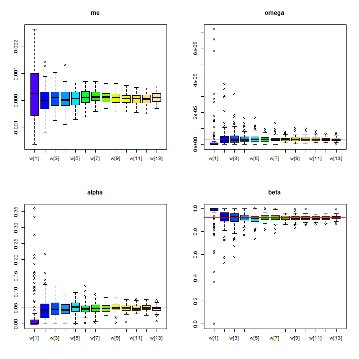
parameter_uncertainty_1


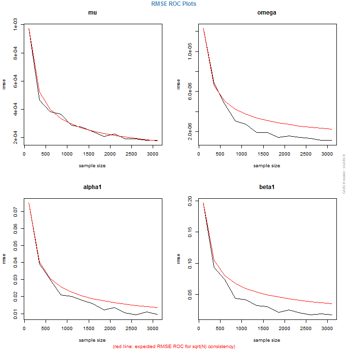
As expected, the standard deviation from the true parameter decreases as the window size increases, with the largest errors for the small window sizes. Another way to see this is via the root mean squared error (RMSE) plots:

plot(mod, which = 4)

parameter_uncertainty_2


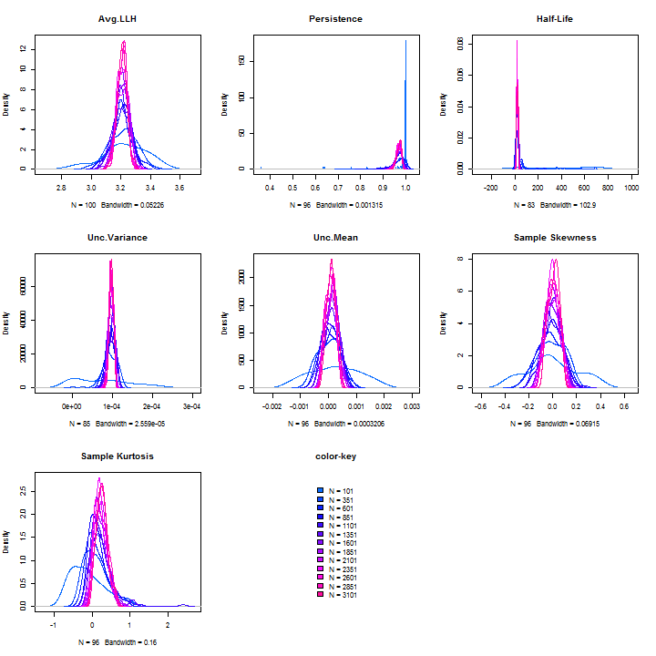
The plots show the RMSE of the fitted versus true coefficients per window size, and the red line the expected RMSE under the assumption of $\sqrt{N}$ consistency. As expected, more (data) leads to less (error). Finally, it it possible to investigate some additional plots showing the distribution of other measures of interest such as persistence, half-life etc:

plot(mod, which = 3)

parameter_uncertainty_3

The ugarchdistribution function makes it easy to investigate the importance of data size on the estimated parameters and provides an initial estimate of the cost of using too little data in GARCH estimation.