This short demonstration illustrates the use of the DCC model and its methods using the rmgarch package, and in particular an alternative method for 2-stage DCC estimation in the presence of the MVT distribution shape (nuisance) parameter. The theoretical background and representation of the model is detailed in the package’s vignette. The dataset and period used are purely for illustration purposes.
library(rmgarch)
library(parallel)
data(dji30retw)
Dat = dji30retw[, 1:10, drop = FALSE]
# define a DCCspec object: 2 stage estimation should usually always use
# Normal for 1-stage (see below for
xspec = ugarchspec(mean.model = list(armaOrder = c(1, 1)), variance.model = list(garchOrder = c(1,1), model = 'eGARCH'), distribution.model = 'norm')
uspec = multispec(replicate(10, xspec))
spec1 = dccspec(uspec = uspec, dccOrder = c(1, 1), distribution = 'mvnorm')
spec1a = dccspec(uspec = uspec, dccOrder = c(1, 1), model='aDCC', distribution = 'mvnorm')
spec2 = dccspec(uspec = uspec, dccOrder = c(1, 1), distribution = 'mvlaplace')
spec2a = dccspec(uspec = uspec, dccOrder = c(1, 1), model='aDCC', distribution = 'mvlaplace')
Since multiple DCC models are being estimated on the same dataset with the same first stage dynamics, we can estimate the first stage once and pass it to the dccfit routine (rather than re-estimating it every time dccfit is called):
cl = makePSOCKcluster(10)
multf = multifit(uspec, Dat, cluster = cl)
Next, the second stage of the DCC model is estimated.
fit1 = dccfit(spec1, data = Dat, fit.control = list(eval.se = TRUE), fit = multf, cluster = cl)
fit1a = dccfit(spec1a, data = Dat, fit.control = list(eval.se = TRUE), fit = multf, cluster = cl)
fit2 = dccfit(spec2, data = Dat, fit.control = list(eval.se = TRUE), fit = multf, cluster = cl)
fit2a = dccfit(spec2a, data = Dat, fit.control = list(eval.se = TRUE), fit = multf, cluster = cl)
To fit the DCC (MVT) model in practice, one either assumes a first stage QML, else must jointly estimate in 1 stage the common shape parameter. In the example that follows below, an alternative approach is used to approximate the common shape parameter.
# First Estimate a QML first stage model (multf already estimated). Then
# estimate the second stage shape parameter.
spec3 = dccspec(uspec = uspec, dccOrder = c(1, 1), distribution = 'mvt')
fit3 = dccfit(spec3, data = Dat, fit.control = list(eval.se = FALSE), fit = multf)
# obtain the multivariate shape parameter:
mvt.shape = rshape(fit3)
# Plug that into a fixed first stage model and iterate :
mvt.l = rep(0, 6)
mvt.s = rep(0, 6)
mvt.l[1] = likelihood(fit3)
mvt.s[1] = mvt.shape
for (i in 1:5) {
xspec = ugarchspec(mean.model = list(armaOrder = c(1, 1)), variance.model = list(garchOrder = c(1,1), model = 'eGARCH'), distribution.model = 'std', fixed.pars = list(shape = mvt.shape))
spec3 = dccspec(uspec = multispec(replicate(10, xspec)), dccOrder = c(1,1), distribution = 'mvt')
fit3 = dccfit(spec3, data = Dat, solver = 'solnp', fit.control = list(eval.se = FALSE))
mvt.shape = rshape(fit3)
mvt.l[i + 1] = likelihood(fit3)
mvt.s[i + 1] = mvt.shape
}
# Finally, once more, fixing the second stage shape parameter, and
# evaluating the standard errors
xspec = ugarchspec(mean.model = list(armaOrder = c(1, 1)), variance.model = list(garchOrder = c(1,1), model = 'eGARCH'), distribution.model = 'std', fixed.pars = list(shape = mvt.shape))
spec3 = dccspec(uspec = multispec(replicate(10, xspec)), dccOrder = c(1, 1), distribution = 'mvt', fixed.pars = list(shape = mvt.shape))
fit3 = dccfit(spec3, data = Dat, solver = 'solnp', fit.control = list(eval.se = TRUE), cluster = cl)
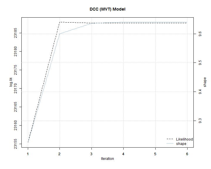
The plot in the change of the likelihood and shape shows that only a few iterations are necessary to converge to a stable value.

The value of the shape parameter implies an excess kurtosis of 1.06. The exercise is repeated for the asymmetric DCC (MVT) model.
xspec = ugarchspec(mean.model = list(armaOrder = c(1,1)), variance.model = list(garchOrder = c(1,1), model = "eGARCH"),  distribution.model = "norm")
spec3a  = dccspec(uspec = multispec( replicate(10, xspec) ), dccOrder = c(1,1), distribution = "mvt", model="aDCC")
fit3a = dccfit(spec3a, data = Dat, fit.control = list(eval.se=FALSE), fit = multf)
# obtain the multivariate shape parameter:
mvtx.shape = rshape(fit3a)
# Plug that into a fixed first stage model and iterate :
mvtx.l = rep(0, 6)
mvtx.s = rep(0, 6)
mvtx.l[1] = likelihood(fit3)
mvtx.s[1] = mvtx.shape
for(i in 1:5){
xspec = ugarchspec(mean.model = list(armaOrder = c(1,1)), variance.model = list(garchOrder = c(1,1), model = "eGARCH"),  distribution.model = "std", fixed.pars = list(shape=mvtx.shape))
spec3a = dccspec(uspec = multispec( replicate(10, xspec) ), dccOrder = c(1,1), model="aDCC", distribution = "mvt")
fit3a = dccfit(spec3a, data = Dat, solver = "solnp", fit.control = list(eval.se=FALSE))
mvtx.shape = rshape(fit3a)
mvtx.l[i+1] = likelihood(fit3a)
mvtx.s[i+1] = mvtx.shape
}
# Finally, once more, fixing the second stage shaoe parameter, and evaluating the standard errors
xspec = ugarchspec(mean.model = list(armaOrder = c(1,1)), variance.model = list(garchOrder = c(1,1), model = "eGARCH"),  distribution.model = "std", fixed.pars = list(shape=mvtx.shape))
spec3a = dccspec(uspec = multispec( replicate(10, xspec) ), dccOrder = c(1,1), model="aDCC", distribution = "mvt", fixed.pars=list(shape=mvtx.shape))
fit3a = dccfit(spec3a, data = Dat, solver = "solnp", fit.control = list(eval.se=TRUE), cluster = cl)
The table below displays the summary of the estimated models, where the stars next to the coefficients indicate the level of significance (*** 1%, ** 5%, * 10%). The asymmetry parameter is everywhere insignificant and, not surprisingly, the MVT distribution provides for the best overall fit (even when accounting for one extra parameter estimated).
##           DCC-MVN   aDCC-MVN    DCC-MVL   aDCC-MVL      DCC-MVT     aDCC-MVT
## a      0.00784*** 0.00639*** 0.00618***  0.0055***   0.00665***    0.00623***
## b      0.97119*** 0.96956*** 0.97624*** 0.97468***   0.97841***    0.97784***
## g                    0.00439               0.00237                 0.00134
## shape                                                9.63947***    9.72587***
## LogLik      22812      22814      22858      22859        23188         23188
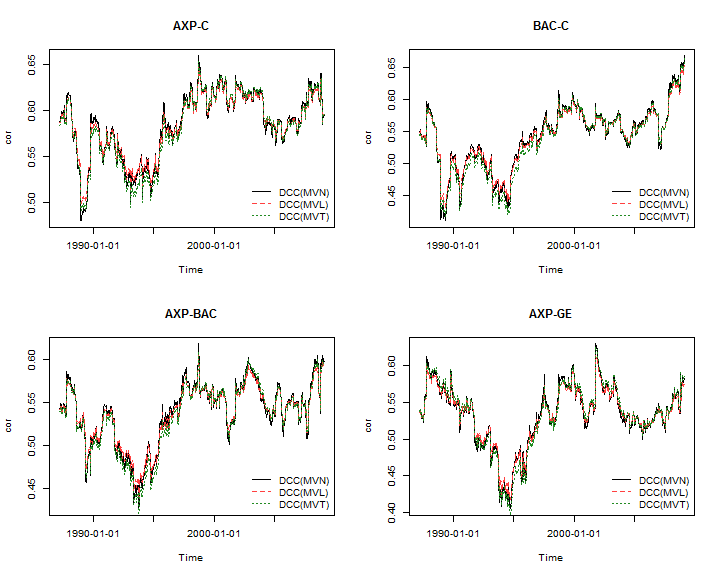
To complete the demonstration, the plots below illustrate some of the dynamic correlations from the different models:

…and remember to terminate the cluster object:
stopCluster(cl)
Would it please be possible to show the code used to visualise those correlations over time? Also if it was so chosen that one of the return series happened to be lagged returns rather than contemporaneous returns, could the correlation values be used in a sort of predictive model?
Hi,
The models only use information at time T-1, so there is no “contemporaneous returns”. You might like to read up on these models, and they are all explained in the vignette of rmgarch (i.e. type vignette(“The_rmgarch_models”, package=”rmgarch”)). The dccforecast routine can create the n-ahead predictions, or you may like to use the dccroll routine for rolling estimation/forecasting instead.
The code for the plots:
library(timeSeries) R1 = rcor(fit1) R2 = rcor(fit2) R3 = rcor(fit3) D = rownames(dji30retw[, 1:10, drop = FALSE]) colx = c(colors()[24], colors()[33], colors()[139]) par(mfrow = c(2,2)) RR = timeSeries(cbind(R1[2,5,],R2[2,5,],R3[2,5,]), D) plot(RR[,1], ylab = "cor", col = colx[1], lty=1 ,lwd=1) for(i in 2:3) lines(RR[,i], col = colx[i], lty = i, lwd=1+i/10) title("AXP-C") legend("bottomright", c("DCC(MVN)", "DCC(MVL)", "DCC(MVT)"), col = colx, lty=1:3, bty="n") RR = timeSeries(cbind(R1[4,5,],R2[4,5,],R3[4,5,]), D) plot(RR[,1], ylab = "cor", col = colx[1], lty=1 ,lwd=1) for(i in 2:3) lines(RR[,i], col = colx[i], lty = i, lwd=1+i/10) title("BAC-C") legend("bottomright", c("DCC(MVN)", "DCC(MVL)", "DCC(MVT)"), col = colx, lty=1:3, bty="n") RR = timeSeries(cbind(R1[2,4,],R2[2,4,],R3[2,4,]), D) plot(RR[,1], ylab = "cor", col = colx[1], lty=1 ,lwd=1) for(i in 2:3) lines(RR[,i], col = colx[i], lty = i, lwd=1+i/10) title("AXP-BAC") legend("bottomright", c("DCC(MVN)", "DCC(MVL)", "DCC(MVT)"), col = colx, lty=1:3, bty="n") RR = timeSeries(cbind(R1[2,10,],R2[2,10,],R3[2,10,]), D) plot(RR[,1], ylab = "cor", col = colx[1], lty=1 ,lwd=1) for(i in 2:3) lines(RR[,i], col = colx[i], lty = i, lwd=1+i/10) title("AXP-GE") legend("bottomright", c("DCC(MVN)", "DCC(MVL)", "DCC(MVT)"), col = colx, lty=1:3, bty="n")Thanks for your response. By lagged return i guess what i meant was in the above data set for example, all Wednesday returns are on the same row. So when this is used as an input to calculate correlation using DCC-GARCH, it will look at simultaneous returns. But if one of the columns included lagged returns instead of simultaneous returns, would the correlation values not now represent the strength of the relationship, between say the return of asset A on Tuesday vs the return of asset B on Wednesday? almost a bit like the first lag of a cross correlation function
Also with regard to the above code for plotting, I get the following error relating to the way that I think you are subsetting your data to get the relevant parts out. But I think I understand what you are doing. Thank you for positing the code up though.
`Error in R1[2, 5, ] : subscript out of bounds`
I think I see what you’re getting at…you want the cross lags (i.e. contagion effect), where the (co)variance of an asset may be influenced by the lagged (co)variance of other assets. Unfortunately, you would need a much more complex MGARCH model than the DCC to obtain this which would then lead to issues of dimensionality and feasibility of estimation. In the DCC model you are estimating the time T correlation of the assets using autoregressive dynamics and shocks at time T-1 from the standardized residuals. The dynamics are driven by a single set of parameters (scalar model), but you also have the possibility to use the Flexible DCC model (FDCC) with group-wise or individual parameters driving the correlation dynamics.
As to the error, I can’t replicate this (it works just fine when I run the code). Please make sure you have the latest version (see the downloads page and get the google code version). To debug check whether R1,R2 and R3 returns arrays, else something may have gone amiss in the code paste or estimation phase.
I’ve also updated the code in the example to show the calculation of the aDCC model which was not shown.
Best,
Alexios
Thanks for the updated code!
I have started to look at potentially fiting it on a rolling basis as well by using dccroll on your example by using the following command but got this error:
fit1 error: convergence problem in univariate fit…
…returning uGARCHmultifit object instead…check and resubmit…
Error: no slot of name “model” for this object of class “uGARCHmultifit”
Is the window too small? or is it something else? Thank again for developing some great packages!
You’ve not provided reproducible code so I can’t comment very much. I also don’t see how you can do what you want with the dccroll
function since the method shown is very customized and not accomodated by dccroll (you need to create your own rolling forecast routine).
Also:
1. Sometimes the dccfit routine does not converge during the 1-stage univariate estimation. This is why you can provide
an already pre-estimated uGARCHmultifit object (which is easy to examine and fine tune for each univariate series estimation) directly
to dccfit (alternatively set solver=”gosolnp” and pray everything goes smoothly).
2. See the rmgarch.tests folder in the tarball distribution for examples.
3. Make sure you have the latest versions from their google repository.
4. Please submit such questions to R-SIG-FINANCE mailing list instead of the blog.
Regards,
Alexios
I have run the asymmetric DCC (MVT) and it seems to work fine. I’ve also managed to plot the results for the covariance/correlation/sigma and so on. I wondered wether there is an easy way to retrieve the values used in the plots (typically sigma and covariance values) to use them in a new data set?
Best regards
Jostein Aaland
Not sure I understand what you mean “use them in a new dataset”.
Have you tried using the “rcov” and “sigma” methods on the estimated objects? Have a look in the rmgarch.tests folder in the src distribution for examples.
Also, make sure you download latest version which contains some fixes to the dcc simulation from the bitbucket repository (see : R-downloads).
Alexios