The interest in high frequency trading and models has grown exponentially in the last decade. While I have some doubts about the validity of any signals emerging from all the noise at higher and higher frequencies, I have nevertheless decided to look at the statistical modelling of intraday returns using GARCH models. Unlike daily and lower frequency returns, intraday data has certain particular characteristics which make the use of standard modelling approaches invalid. For the purpose of this article, I will use 1-min returns for Citigroup for the period 02-Jan-2008 to 29-Feb-2008, which is available to download here with permission from QuantQuote. This dataset is supplied dividend and split adjusted and with outliers removed. The intraday time range considered is 09:30 to 16:00, the official NYSE trading hours. As with most such studies on intraday data modelling, the first return of the day is removed. Daily data for the symbol is downloaded from Yahoo finance.
library(rugarch)
Sys.setenv(TZ = 'GMT')
library(quantmod)
R_i = read.csv('C_2008_1minret.csv')
R_i = xts(R_i[, 2], as.POSIXct(R_i[, 1]))
C = quantmod::getSymbols('C', from = '2000-01-01',auto.assign=FALSE)
C = quantmod::adjustOHLC(C, use.Adjusted = TRUE)
R_d = TTR::ROC(Cl(C), na.pad = FALSE)
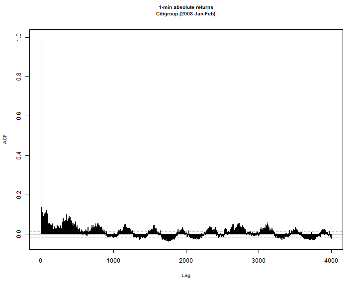
Consider the correlogram of the absolute 1-min returns for Citigroup during the sample period in question:
par(cex.main = 0.85, col.main = 'black')
acf(abs(as.numeric(R_i)), lag.max = 4000, main = '1-min absolute returns\nCitigroup (2008 Jan-Feb)', cex.lab = 0.8)
The regular pattern is quite clear, repeating approximately every 390 periods (1-day) and showing an increase in volatility around the opening and closing times. GARCH, and more generally ARMA type models can only handle an exponential decay, and not the type of pattern seen here. Several approaches have been suggested in the literature in order to de-seasonalize the absolute returns such as the flexible Fourier method of Andersen and Bollerslev (1997), and the periodic GARCH model of Bollerslev and Ghysels (1996). Unfortunately I have found none of these, or closely related models particularly easy to work with. More recently, Engle and Sokalska (2012) (henceforth ES2012) introduced the multiplicative component GARCH model as a parsimonious alternative, which I have now included in the rugarch package (ver 1.01-6). This article discusses its implementation, challenges and specific details of working with this model, which allows a rather simple but powerful way to use GARCH for regularly spaced intraday returns.
The Model
Consider the continuously compounded return \( r_{t,i} \), where \( t \) denotes the day and \( i \) the regularly spaced time interval at which the return was calculated. Under this model, the conditional variance is a multiplicative product of daily, diurnal and stochastic (intraday) components, so that the return process may be represented as:
\[ \begin{gathered}
{r_{t,i}} = {\mu _{t,i}} + {\varepsilon _{t,i}}\\
{\varepsilon _{t,i}} = \left( {{q_{t,i}}{\sigma _t}{s_i}} \right){z_{t,i}}
\end{gathered} \]
where \( q_{t,i} \) is the stochastic intraday volatility, \( \sigma_t \) a daily exogenously determined forecast volatility, \( s_i \) the diurnal volatility in each regularly spaced interval \( i \), \( z_{t,i} \) the i.i.d (0,1) standardized innovation which conditionally follows some appropriately chosen distribution. In ES2012, the forecast volatility \( \sigma_t \) is derived from a multifactor risk model externally, but it is just as possible to generate such forecasts from a daily GARCH model. The seasonal (diurnal) part of the process is defined as:
\[ {s_i} = \frac{1}{T}\sum\limits_{t = 1}^T {\left( {\varepsilon _{_{t,i}}^2/\sigma _t^2} \right)}. \]
Dividing the residuals by the diurnal and daily volatility gives the normalized residuals (\( \bar\varepsilon \)):
\[ {{\bar \varepsilon }_{t,i}} = {\varepsilon _{t,i}}/\left( {{\sigma _t}{s_i}} \right) \]
which may then be used to generate the stochastic component of volatility \( q_{t,i} \) with GARCH motion dynamics. In the rugarch package, unlike the paper of ES2012, the conditional mean and variance equations (and hence the diurnal component on the residuals from the conditional mean filtration) are estimated jointly. Furthermore, and unlike ES2012, it is possible to include ARMAX dynamics in the conditional mean, though because of the complexity of the model and its use of time indices, ARCH-m is not currently allowed. Finally, as an additional departure from ES2012, the diurnal component in the rugarch package is estimated using the median rather than the mean function (since version 1.2-3), providing a more robust alternative given the type and length of the data typically used. The next sections provide a demonstration of the model using the Citigroup dataset.
Estimation
Unlike all other GARCH models implemented in rugarch, the mcsGARCH model requires the user to pass an xts object of the forecast daily variance of the data for the period under consideration.
# Find the unique days in the intraday sample
n = length(unique(format(index(R_i), '%Y-%m-%d')))
# define a daily spec
spec_d = ugarchspec(mean.model = list(armaOrder = c(1, 1)), variance.model = list(model = 'eGARCH', garchOrder = c(2, 1)), distribution = 'nig')
# use the ugarchroll method to create a rolling forecast for the period in
# question:
roll = ugarchroll(spec_d, data = R_d['/2008-02-29'], forecast.length = n, refit.every = 5, refit.window = 'moving', moving.size = 2000, calculate.VaR = FALSE)
# extract the sigma forecast
df = as.data.frame(roll)
f_sigma = as.xts(df[, 'Sigma', drop = FALSE])
# now estimate the intraday model
spec = ugarchspec(mean.model = list(armaOrder = c(1, 1), include.mean = TRUE), variance.model = list(model = 'mcsGARCH'), distribution = 'nig')
# DailyVar is the required xts object of the forecast daily variance
fit = ugarchfit(data = R_i, spec = spec, DailyVar = f_sigma^2)
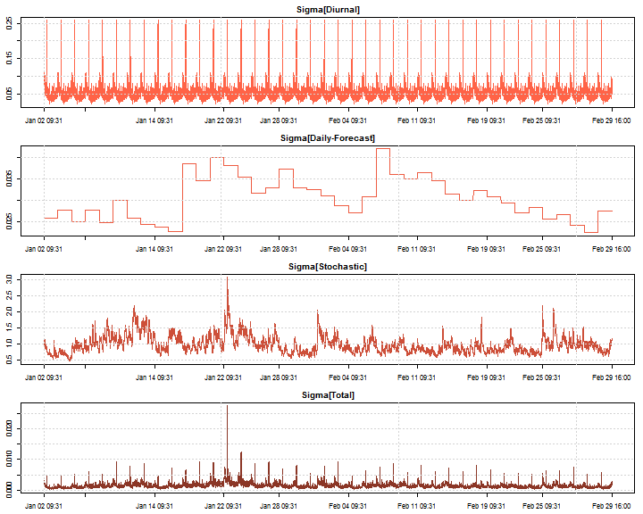
The following plots show the decomposition of the volatility into its various components. The regular pattern of the Total volatility would have been impossible to capture using standard GARCH models. Note that although the volatility series are stored as xts objects, they cannot be properly plotted using the standard plot.xts function which is why I make use of the axis function with a numeric series.
ep < - axTicksByTime(fit@model$DiurnalVar)
par(mfrow = c(4, 1), mar = c(2.5, 2.5, 2, 1))
plot(as.numeric(fit@model$DiurnalVar^0.5), type = 'l', main = 'Sigma[Diurnal]', col = 'tomato1', xaxt = 'n', ylab = 'sigma', xlab = ' ')
axis(1, at = ep, labels = names(ep), tick = TRUE)
grid()
plot(as.numeric(fit@model$DailyVar^0.5), type = 'l', main = 'Sigma[Daily-Forecast]', col = 'tomato2', xaxt = 'n', ylab = 'sigma', xlab = ' ')
axis(1, at = ep, labels = names(ep), tick = TRUE)
grid()
plot(fit@fit$q, type = 'l', main = 'Sigma[Stochastic]', col = 'tomato3', xaxt = 'n', ylab = 'sigma', xlab = ' ')
axis(1, at = ep, labels = names(ep), tick = TRUE)
grid()
plot(as.numeric(sigma(fit)), type = 'l', main = 'Sigma[Total]', col = 'tomato4', xaxt = 'n', ylab = 'sigma', xlab = ' ')
axis(1, at = ep, labels = names(ep), tick = TRUE)
grid()
Forecasting
The biggest challenge in writing code for the forecast was dealing with the aligning and matching of times, particularly future time/dates, since the model depends on the diurnal component which is time specific. As a key component of the forecast routine, I wrote a little function which creates a sequence of time/dates, similar to seq.POSIXt, but with the extra option of defining the time interval which dictates the start and end of the trading day. For example, considering the opening and closing times of the NYSE, 09:30 to 16:00, I would like to be able to create a set of n future periods starting from T0 within only this interval, and excluding weekends. The function is defined as:
ftseq(T0, length.out, by, interval, exclude.weekends = TRUE)
where T0 is a POSIXct date/time of the starting period, length.out the periods ahead to consider, by the difftime (e.g. “mins”), and interval a character vector of the start and end times which T0 must belong to and is a multiple of by.
# create the interval
interval = format(seq(as.POSIXct('2008-01-02 09:31:00'), as.POSIXct('2008-01-02 16:00:00'), by = 'min'), '%H:%M:%S')
#
ForcTime = ftseq(T0 = as.POSIXct('2008-02-29 16:00:00'), length.out = 390 * 2 + 1, by = 'mins', interval = interval)
tail(ForcTime, 25)
##  [1] '2008-03-04 15:37:00 GMT' '2008-03-04 15:38:00 GMT'
##  [3] '2008-03-04 15:39:00 GMT' '2008-03-04 15:40:00 GMT'
##  [5] '2008-03-04 15:41:00 GMT' '2008-03-04 15:42:00 GMT'
##  [7] '2008-03-04 15:43:00 GMT' '2008-03-04 15:44:00 GMT'
##  [9] '2008-03-04 15:45:00 GMT' '2008-03-04 15:46:00 GMT'
## [11] '2008-03-04 15:47:00 GMT' '2008-03-04 15:48:00 GMT'
## [13] '2008-03-04 15:49:00 GMT' '2008-03-04 15:50:00 GMT'
## [15] '2008-03-04 15:51:00 GMT' '2008-03-04 15:52:00 GMT'
## [17] '2008-03-04 15:53:00 GMT' '2008-03-04 15:54:00 GMT'
## [19] '2008-03-04 15:55:00 GMT' '2008-03-04 15:56:00 GMT'
## [21] '2008-03-04 15:57:00 GMT' '2008-03-04 15:58:00 GMT'
## [23] '2008-03-04 15:59:00 GMT' '2008-03-04 16:00:00 GMT'
## [25] '2008-03-05 09:31:00 GMT'
As can be seen, the first time is immediately after T0 (T0 is not included), and the sequence only runs for the defined interval, and optionally (default TRUE) skips weekends. This comes in very handy in the forecast routine.
Like the estimation method, the forecast routine also requires that you supply the forecast volatility for the period under consideration. However, because of the possible use of the out.sample in the estimation routine, it is not known beforehand whether this will eventually be needed since there may be enough intraday data in the out.sample period and the combination of n.ahead+n.roll chosen so that this user supplied forecast is not required. If you do not supply it and it is needed the routine will check and let you know with an error message. Finally, the presence of the diurnal component complicates the long run unconditional forecast of the underlying variance, so that the use of the uncvariance and related methods will always return the value for the component variance rather than the actual total variance (unlike the csGARCH model which returns both).
fit2 = ugarchfit(data = R_i, spec = spec, DailyVar = f_sigma^2, out.sample = 300)
# won't supply DailyVar to get an error
forc = ugarchforecast(fit2, n.ahead = 10, n.roll = 299)
## Error: DailyVar requires forecasts for: 2008-03-03 ...resubmit.
Notice the error which indicates we need 2008-03-03 forecast. Since we don’t have it, we re-estimate with ugarchforecast:
fit_d = ugarchfit(spec_d, data = R_d['2002/2008-02-29'])
forc_d = ugarchforecast(fit_d, n.ahead = 1)
f_sigma = xts(as.numeric(sigma(forc_d)), as.POSIXct('2008-03-03'))
# intraday forecast
forc = ugarchforecast(fit2, n.ahead = 10, n.roll = 299, DailyVar = f_sigma^2)
show(forc)
##
## *------------------------------------*
## *       GARCH Model Forecast         *
## *------------------------------------*
## Model: mcsGARCH
## Horizon: 10
## Roll Steps: 299
## Out of Sample: 10
##
## 0-roll forecast [T0=2008-02-29 11:00:00]:
##          Series Sigma[Total] Sigma[Stochastic]
## T+1  -7.681e-06    0.0015132            0.8702
## T+2  -7.664e-06    0.0057046            0.8718
## T+3  -7.657e-06    0.0055551            0.8734
## T+4  -7.654e-06    0.0058834            0.8750
## T+5  -7.653e-06    0.0063295            0.8766
## T+6  -7.653e-06    0.0013036            0.8781
## T+7  -7.653e-06    0.0012846            0.8797
## T+8  -7.653e-06    0.0011227            0.8812
## T+9  -7.652e-06    0.0008177            0.8827
## T+10 -7.652e-06    0.0009259            0.8842
Note that plot methods for this model are not yet fully implemented for reasons described previously.
Simulation
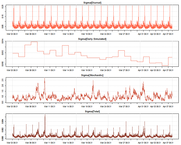
Unlike standard GARCH simulation, the interval time is important in intraday GARCH since we are generating paths which follow very specific regularly sampled time points. Additionally, simulated or forecast daily variance needs to again be supplied for the simulation period under consideration. This is an xts object, and can also optionally have m.sim columns so that each independent simulation is based on the adjusted residuals by an independent simulation of the daily variance. The following example code shows the simulation of 10,000 points at 1-min intervals into the future and illustrates the effect of the seasonality component:
T0 = tail(index(R_i), 1)
# model$dtime contains the set of unique interval points in the dataset
# (and available from all rugarch objects for the mcsGARCH model)
# model$dvalues contains the diurnal component for each interval
ftime = ftseq(T0, length.out = 10000, by = fit@model$modeldata$period, interval = fit@model$dtime)
dtime = unique(format(ftime, '%Y-%m-%d'))
#
sim_d = ugarchsim(fit_d, n.sim = length(dtime), m.sim = 1)
var_sim = xts(as.matrix(sigma(sim_d)^2), as.POSIXct(dtime))
sim = ugarchsim(fit, n.sim = 10000, n.start = 0, m.sim = 1, DailyVar = var_sim, rseed = 10)
#
ep < - axTicksByTime(sim@simulation$DiurnalVar)
par(mfrow = c(4, 1), mar = c(2.5, 2.5, 2, 1))
plot(as.numeric(sim@simulation$DiurnalVar^0.5), type = 'l', main = 'Sigma[Diurnal]', col = 'tomato1', xaxt = 'n', ylab = 'sigma', xlab = ' ')
axis(1, at = ep, labels = names(ep), tick = TRUE)
grid()
plot(as.numeric(sim@simulation$DailyVar^0.5), type = 'l', main = 'Sigma[Daily-Simulated]', col = 'tomato2', xaxt = 'n', ylab = 'sigma', xlab = ' ')
axis(1, at = ep, labels = names(ep), tick = TRUE)
grid()
plot(sim@simulation$qSim[, 1], type = 'l', main = 'Sigma[Stochastic]', col = 'tomato3', xaxt = 'n', ylab = 'sigma', xlab = ' ')
axis(1, at = ep, labels = names(ep), tick = TRUE)
grid()
plot(as.numeric(sigma(sim)), type = 'l', main = 'Sigma[Total]', col = 'tomato4',
xaxt = 'n', ylab = 'sigma', xlab = ' ')
axis(1, at = ep, labels = names(ep), tick = TRUE)
grid()
A rolling backtest and Value at Risk
The ugarchroll function is quite useful for testing a model’s adequacy in a backtest application, and the code below illustrates this for the mcsGARCH model for the data and period under consideration.
n = length(index(R_d['2008-01-01/2008-03-01']))
spec_d = ugarchspec(mean.model = list(armaOrder = c(1, 1)), variance.model = list(model = 'sGARCH'), distribution = 'std')
roll = ugarchroll(spec_d, data = R_d['/2008-02-29'], forecast.length = n, refit.every = 5, refit.window = 'moving', moving.size = 2000, calculate.VaR = FALSE)
df = as.data.frame(roll)
f_sigma = as.xts(df[, 'Sigma', drop = FALSE])
spec = ugarchspec(mean.model = list(armaOrder = c(1, 1), include.mean = TRUE), variance.model = list(model = 'mcsGARCH'), distribution = 'std')
roll = ugarchroll(spec, data = R_i, DailyVar = f_sigma^2, forecast.length = 3000, refit.every = 390, refit.window = 'moving', moving.size = 3000, calculate.VaR = TRUE)
# Generate the 1% VaR report
report(roll)
## VaR Backtest Report
## ===========================================
## Model: mcsGARCH-std
## Backtest Length: 3000
## ==========================================
## alpha:             1%
## Expected Exceed:   30
## Actual VaR Exceed: 33
## Actual %:          1.1%
##
## Unconditional Coverage (Kupiec)
## Null-Hypothesis: Correct Exceedances
## LR.uc Statistic: 0.294
## LR.uc Critical:  3.841
## LR.uc p-value:   0.588
## Reject Null:     NO
##
## Conditional Coverage (Christoffersen)
## Null-Hypothesis: Correct Exceedances and
##                  Independence of Failures
## LR.cc Statistic: 1.028
## LR.cc Critical:  5.991
## LR.cc p-value:   0.598
## Reject Null:     NO
Not bad at all. Who say’s GARCH models are not good!?
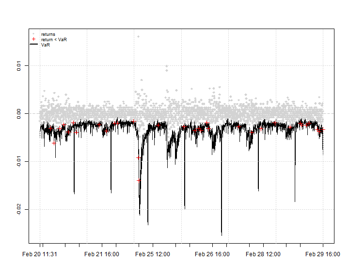
The VaRplot function has been adjusted to work nicely with intraday data as shown below. The spikes in the VaR observed are the result of the seasonal component around the opening of trading.
D = as.POSIXct(rownames(roll@forecast$VaR))
VaRplot(0.01, actual = xts(roll@forecast$VaR[, 3], D), VaR = xts(roll@forecast$VaR[,1], D))
Further Developments
It is quite ‘easy’ to add additional GARCH flavors to the multiplicative model such as the eGARCH, GJR etc, and might do so in due course, time permitting. Another possible direction for expansion would be to treat the diurnal effect separately for each day of the week. I estimate that this would not be too hard to implement, providing a marginal slowdown in the estimation as a result of the increased lookup time for the matching of time and days.
Finally, this model is not ‘plug-and-play’, requiring some thought in the use of time & dates, and the preparation of the intraday returns. The garbage-in garbage-out rule clearly applies.
Please remember that questions about this or other issues with rugarch should be addressed to the r-sig-finance mailing list.
References
Bollerslev, T., & Ghysels, E. (1996). Periodic autoregressive conditional heteroscedasticity. Journal of Business & Economic Statistics, 14(2), 139–151.
Andersen, T. G., & Bollerslev, T. (1997). Intraday periodicity and volatility persistence in financial markets. Journal of Empirical Finance, 4(2), 115–158.
Engle, R. F., & Sokalska, M. E. (2012). Forecasting intraday volatility in the US equity market. Multiplicative component GARCH. Journal of Financial Econometrics, 10(1), 54–83.


