In a previous post, I provided a brief intro to the exponentially weighted moving average (EWMA) volatility as a restricted iGARCH model. In this post I generalize to the multivariate case and add some additional flavor by considering a diagonal EWMA covariance model with the possibility of centering by the EWMA mean of the variables.
Consider the following model for the evolution of the covariance matrix: \[
{\Sigma _t} = \left( {1 – \lambda } \right)\left( {{r_{t – 1}} – \mu } \right){\left( {{r_t} – \mu } \right)^\prime } + \lambda {\Sigma _{t – 1}}
\] where \(\lambda\) is the decay factor as discussed in the previous post, or equivalently the persistence parameter. The model is again a restricted multivariate iGARCH model with the restritions of zero intercept and scalar dynamics for the covariance (in addition to the iGARCH restriction of \(\alpha=1-\beta\)). The rmgarch package already includes estimation for some multivariate feasible GARCH models, but here instead I am not concerned with estimation but with fast calculation or filtering using pre-specified values. Without complicating matters too much, we can extend this model to include seperate dynamics for each variable in addition to the use of EWMA model for the mean (and stop short of specifying full dynamics in this non-estimation based setting). The model then becomes: \[
\begin{gathered}
{\Sigma _t} = \left( {{\mathbf{1}} – {{\mathbf{\lambda }}_v}} \right)\left( {{r_{t – 1}} – {\mu _{t}}} \right){\left( {{r_t} – {\mu _{t}}} \right)^\prime }{\left( {{\mathbf{1}} – {{\mathbf{\lambda }}_v}} \right)^\prime } + {{\mathbf{\lambda }}_v}{\Sigma _{t – 1}}{{{\mathbf{\lambda ‘}}}_v} \\
{\mu _t} = \left( {{\mathbf{1}} – {{\mathbf{\lambda }}_r}} \right){r_{t – 1}} + {{\mathbf{\lambda }}_r}{\mu _{t – 1}} \\
\end{gathered}
\] where \({{\mathbf{\lambda }}_v} = diag\left( {{\lambda _{v,1}},…,{\lambda _{v,m}}} \right)\) is a matrix of the diagonal entries of the covariance decay parameters, \({{\mathbf{\lambda }}_r} = \left( {{\lambda _{r,1}},…,{\lambda _{r,m}}} \right)^\prime\) the vector of decay parameters for the EWMA model of the mean (which collapses to the standard case when they are all 1), and 1 a diagonal matrix of ones for the \(\Sigma_t\) case and a vector of ones for the \(\mu_t\) case. Finally, initialization of the recursion uses the unconditional values i.e. the sample mean and covariance matrix of the dataset.
Since the title of the post is about fast filtering, it is really not going to be very efficient to code this in R. Instead, the code below provides an inline Rcpp+Armadillo implementation:
library(inline)
require(RcppArmadillo)
dewmacov <- cxxfunction( signature(X = "matrix", vlambda = "matrix", mlambda = "numeric") , '
    arma::mat Z = Rcpp::as<arma::mat>(X);
    int n = (int) Z.n_rows;
    int m = (int) Z.n_cols;
    arma::mat vlam = Rcpp::as<arma::mat>(vlambda);
    arma::mat vmal = arma::eye(m,m) - vlam;
    arma::rowvec mlam = Rcpp::as<arma::rowvec>(mlambda);
    arma::rowvec mmal = arma::ones(1,m) - mlam;
    arma::cube C(m,m,n);
    arma::mat M(n,m);
    arma::mat initC = arma::cov(Z,1);
    arma::rowvec initM = arma::mean(Z);
    int i;
    C.slice(0) = vlam*initC*arma::trans(vlam);
    M.row(0) = mlam % initM;
    for(i=1;i<n;i++){
    M.row(i) = mmal % Z.row(i-1) + mlam % M.row(i-1);
    C.slice(i) = vmal*( arma::trans(Z.row(i-1)-M.row(i))*(Z.row(i-1)-M.row(i)) )*arma::trans(vmal)+vlam*C.slice(i-1)*arma::trans(vlam);
    }
    return wrap( C ) ;
', plugin = "RcppArmadillo" )
sewmacov <- cxxfunction( signature(X = "matrix", vlambda = "numeric") , '
  arma::mat Z = Rcpp::as<arma::mat>(X);
    int n = (int) Z.n_rows;
    int m = (int) Z.n_cols;
  double vlam = Rcpp::as<double>(vlambda);
    double vmal = 1.0 - vlam;
    arma::cube C(m,m,n);
    arma::mat initC = arma::cov(Z,1);
    int i;
    C.slice(0) = vlam*initC;
    for(i=1;i<n;i++){
        C.slice(i) = vmal*(arma::trans(Z.row(i-1))*Z.row(i-1))+vlam*C.slice(i-1);
    }
    return wrap( C ) ;
  ', plugin = "RcppArmadillo" )
# A cov2cor function for arrays
cv2cr = cxxfunction(signature(x = "vector", n = "integer"), '
  Rcpp::NumericVector XX(x);
  Rcpp::IntegerVector dim(n);
  arma::cube AY(XX.begin(), dim[0], dim[1], dim[2]);
  arma::cube AX(dim[0], dim[1], dim[2]);
    int i;
    arma::mat tmp(dim[0], dim[1]);
    for(i=0;i<dim[2];i++){
        tmp = arma::diagmat(1/arma::sqrt(diagvec(AY.slice(i))));
        AX.slice(i) = tmp * AY.slice(i) * tmp.t();
    }
  return(wrap(AX));
', plugin = "RcppArmadillo" )
# wrapper for passing the array dimensions
cov2cor2 = function(x)
{
  n = dim(x)
  return(cv2cr(x, n))
}
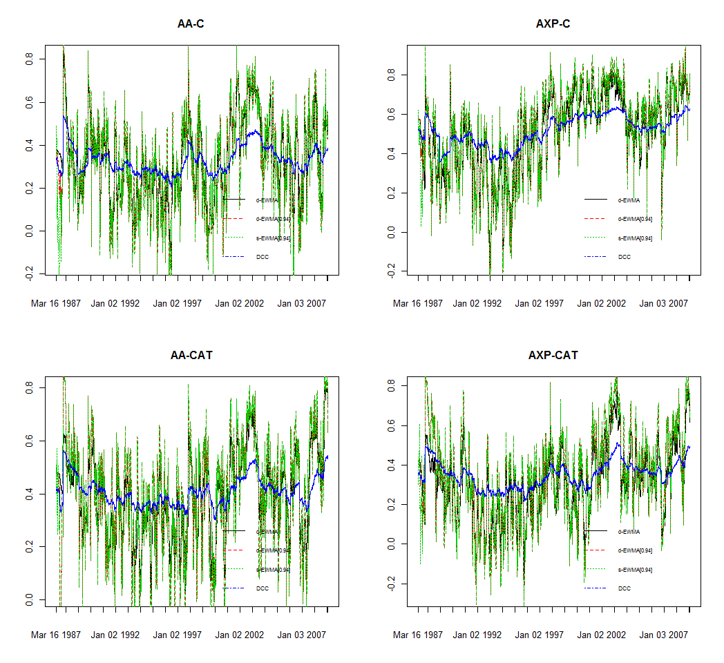
I’ve not included any checks, this is a raw function which you need to use with caution. I’ve also included the simpler scalar case to compare to the diagonal as a quick check and for cases when the diagonal is not needed (which would make some calculations redundant). In the following example I estimate a DCC model and compare with the scalar and diagonal EWMA models.
library(rmgarch)
library(xts)
data(dji30ret)
X = as.xts(dji30ret)
cn = colnames(X)
spec = ugarchspec(mean.model=list(armaOrder=c(0,0)),variance.model=list(model='iGARCH'), fixed.pars=list(omega=0))
vlambda = apply(X, 2, function(x) coef(ugarchfit(spec, x))['beta1'])
mlambda = rep(1, 30)
V1 = dewmacov(coredata(X), diag(sqrt(vlambda)), mlambda)
V2 = dewmacov(coredata(X), diag(rep(sqrt(0.94), 30)), mlambda)
V3 = sewmacov(scale(coredata(X), scale=FALSE), 0.94)
R1 = cov2cor2(V1)
R2 = cov2cor2(V2)
R3 = cov2cor2(V3)
# compare to DCC:
mspec = dccspec(multispec(replicate(30, ugarchspec(variance.model=list(variance.targeting=TRUE),mean.model=list(armaOrder=c(0,0))))))
mfit = dccfit(mspec, X,  fit.control = list(eval.se = FALSE))
R4 = rcor(mfit)
cm=expand.grid(1:2,5:6)
par(mfrow=c(2,2))
for(i in 1:4){
  plot(xts(R1[cm[i,1],cm[i,2],], index(X)), main=paste(cn[cm[i,1]],'-',cn[cm[i,2]],sep=''), auto.grid = FALSE, minor.ticks = FALSE)
  lines(xts(R2[cm[i,1],cm[i,2],], index(X)), col=2, lty=2)
  lines(xts(R3[cm[i,1],cm[i,2],], index(X)), col=3, lty=3)
  lines(xts(R4[cm[i,1],cm[i,2],], index(X)), col=4, lwd=1.5)
  legend('bottomright', c('d-EWMA','d-EWMA[0.94]','s-EWMA[0.94]','DCC'), col=c(1,2,3,4), cex=0.6, lty=1:4, bty='n')
}
The DCC persistence parameter (dcc_beta) is very high (>0.99), while the shock parameter (dcc_alpha) quite low. This is reflected in the rather smooth correlation seen in the plot for the DCC model, whereas for the EWMA using pre-determined values the variation is much higher. Why the dcc parameter shock value is so low is not clear at the moment, but may be related to any number of factors including inadequate centering (no AR dynamics), outliers, or failure to adequately scale the standardized residuals using first stage vanilla GARCH dynamics. However, this was not the purpose of this post, but instead to provide a quick outline of the EWMA covariance model.
