In the last few years there has been a increasing tendency to ignore the value of a disciplined quantitative approach to the portfolio allocation process in favor of simple and static weighting schemes such as equal weighting or some type of adjusted volatility weighting. The former simply ignores the underlying security dynamics, assuming equal risk-return, whilst the latter assumes risk is equal to variance in which case it also ignores covariance between securities and other pertinent features of observed security dynamics. It is true that a simplified approach is easier to explain to clients (and easier to understand by most practitioners), and may be justified in cases when there is little data available for modelling the underlying dynamics.
In a much cited paper DeMiguel, Garlappi, and Uppal (2009) argued that it is difficult to beat the equal weighting strategy, considering a number of mostly mean-variance related models on limited history monthly data. The premise of their argument was based on the uncertainty in estimation of quantities such as covariance. While it is certainly true that uncertainty about such quantities is related to the size of the dataset, using a very short history of monthly data to make that point and publish the paper does not appear to me to provide for a scholarly answer to the paper’s title (“Optimal Versus Naive Diversification: How Inefficient is the 1/N Portfolio Strategy?”). Additionally, they do not even test the significance in the difference of the Sharpe ratios which makes it rather difficult to draw any conclusions.
In defense of optimization, and a direct reply to that study, which was criticized for using very short histories for the estimation of the covariance, Kritzman, Page, and Turkington (2010) provide a very thorough empirical application across a number of portfolios using the mean-variance criterion, including one comprising daily returns of the point in time constituents of the S&P500 from 1998 to 2008, and show substantially large differences (though again not statistically tested) in Sharpe ratios against the equal weighting strategy. The arguments against 1/N are readily generalized to any static weight allocation scheme, such as employed by most benchmark indices, with clear implications for benchmark policy choice and investment manager reward schemes. The question of the efficiency of benchmark indices was addressed some time ago by Grinold (1992) who asked whether index benchmarks are efficient, using the test of Gibbons, Ross, and Shanken (1989) on the country indices of Australia, Germany, Japan, U.K. and U.S. for the period ending 1991 (with start dates as early as 1973 for the U.S.). He found that 4 out of the 5 indices were not efficient ex-post. More recently, Demey, Maillard, and Roncalli (2010) also argued that neither capitalization nor price weighted indices are efficient, exposing investors to what should be diversifiable risk.
In this blog article, I will try to provide one empirical application, using a popular Global Tactical Asset Allocation model based on an approach proposed by Faber(2007), to show the value of a quantitive approach to asset allocation over the naive 1/N strategy. I make use of the rmgarch and parma packages, together with the blotter package for realistic portfolio accounting. Because of the complexity of the setup, the code to generate the tables and figures will be provided seperately as a link (see bottom of page) rather than displayed inline and there are a number of custom functions written on top of blotter. While the quantstrat package provides one excellent avenue for implementing such strategies, I have not used it in this case, opting for a more custom solution which provides for more transparency in what is actually happening under the hood. Feel free to drop me a note if you find any errors or have any suggestions.
Data Universe Setup
One of the issues in many of the backtests one reads about is a failure to take into account companies which have delisted. This leads to the so called survivorship bias problem when backtesting equities, and is even more pronounced in hedge fund databases where reporting is voluntary (e.g. funds which do badly in one year may decide not to report). A realistic test of the efficiency of a benchmark index would require having access to the point in time constituents of that index, which would probably require access to a proprietary database. In this application, I will instead consider a set of market aggregates, which alleviates this problem, and also provides for two additional benefits. First, the implementation of the strategy becomes scalable and there are no issues of liquidity (for most of the indices), and second, the use of aggregates eliminates some of the idiosyncratic noise found in individual securities which enables the identification of trends using a moving average filter much easier. Because ETF’s usually have a limited history going back to the early 2000’s, I have opted to use where appropriate a Vanguard fund as the instrument of choice for testing. Nevertheless, almost half of the securities do not trade for most of 1990 and early 2000 making it a little difficult to draw firm conclusions for the whole period since portfolio optimization benefits from a large and diversified group of securities.
The universe is comprised of the following assets:
- VFINX (US Equity s:1987), VEURX (EU Equity s:1990), VPACX (Asia Pacific Equity s:1990), VEIEX (Emerging Market Equity s:1995)
- SH (ProShares Short S&P 500 s:2006)
- VGSIX (REIT s:1996)
- IXC (Global Energy s:2001), GLD (Gold s:2004)
- VWEHX (High Yield Corporate s:1989), VCLT (Long Term Corporate s:2009)
- DBV (Carry Trade G10 s:2006)
This represents a select exposure to global Equities, US Corporates, Commodities, US Real Estate and Rates/Currencies. The use of the Short S&P 500 index is to obtain some additional diversification in times of global crises, since the strategy is long only.
Data Universe Characteristics
A first look at some of the statistics of this dataset reveals that it exhibits the typical set of stylized facts.
| Ticker | Mean | Median | Min | Max | Stdev | Skewness | Kurtosis | LB(1) | LB(2) | ARCH-LM(1) | JB |
|---|---|---|---|---|---|---|---|---|---|---|---|
| VFINX | 0.0003 | 0.0007 | -0.2286 | 0.1096 | 0.012 | -1.2924 | 30.34 | 0.0001 | 0 | 0 | 0 |
| VEURX | 0.0003 | 0.0008 | -0.1091 | 0.1174 | 0.0132 | -0.3212 | 11.367 | 0.0137 | 0.0011 | 0 | 0 |
| VPACX | 0.0001 | 0 | -0.0856 | 0.1277 | 0.0134 | 0.2265 | 9.119 | 0.3344 | 0.0758 | 0 | 0 |
| VEIEX | 0.0003 | 0.0011 | -0.126 | 0.1367 | 0.0146 | -0.3943 | 13.32 | 0 | 0 | 0 | 0 |
| SH | -0.0004 | -0.0008 | -0.1168 | 0.09 | 0.0146 | -0.1571 | 12.154 | 0 | 0 | 0 | 0 |
| VGSIX | 0.0004 | 0 | -0.2149 | 0.169 | 0.0184 | -0.2011 | 23.696 | 0 | 0 | 0 | 0 |
| IXC | 0.0004 | 0.001 | -0.1412 | 0.1434 | 0.0173 | -0.3857 | 12.174 | 0.0021 | 0 | 0 | 0 |
| GLD | 0.0005 | 0.0008 | -0.0919 | 0.107 | 0.0131 | -0.3751 | 8.728 | 0.4471 | 0.7443 | 0 | 0 |
| VWEHX | 0.0003 | 0 | -0.0521 | 0.0231 | 0.0032 | -0.6722 | 21.772 | 0 | 0 | 0 | 0 |
| VCLT | 0.0003 | 0.0006 | -0.0352 | 0.0224 | 0.0064 | -0.2832 | 4.768 | 0.0067 | 0.0218 | 0.0003 | 0 |
| DBV | 0 | 0.0006 | -0.085 | 0.0642 | 0.0097 | -0.7927 | 14.815 | 0.0001 | 0.0003 | 0 | 0 |
There is serial correlation (Ljung-Box test) and ARCH effects (ARCH-LM test) in addition to clear rejection of normality (Jarque-Bera test). This is of course not surprising for daily returns, though the question of such effects at lower frequencies is debatable (there is usually not enough data to form adequate tests, whilst aggregation methods require a host of additional assumptions e.g. weak GARCH etc). Given the presence of such such dynamics in the dataset, with varying degrees of skewness and kurtosis across the securities, it is certainly not reasonable to opt for a 1/N approach to the allocation of capital.
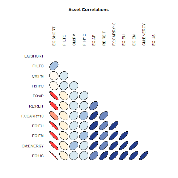
The figure shows the pairwise complete correlations of the securities used in this application which range from the highly correlated (Equities, Energy, REITS and Carry Trade) to the low correlation (Fixed Income and Precious Metals) and the negatively correlated (Equity Short).
The Modelling and Optimization Process
There are 2 competing considerations to take into account when modelling security dynamics and the generation of forecasts. Obviously, more data is preferred to less when using such models as GARCH in order to obtain good estimates of the persistence. On the other hand, the higher the frequency of the data the more the noise in any signal generating mechanism such as the moving average system. In addition, we want to optimize and rebalance based on a lower frequency (monthly) basis so as to eliminate transaction costs and turnover. The signal generating mechanism I apply is based on the crossover of a slow and fast exponential moving average on monthly prices, the length of which is determined dynamically at each point in time. This filter is applied to all securities with a minimum of 600 daily data points, and those with a positive signal are then considered part of the modelling universe. If there are 3 or less securities in the universe, the optimization is not undertaken and instead a fixed weight is assigned to each security (and this may add up to less than 100% investment). The modelling of the universe of positive signal prospects is undertaken using an AR(1)-GARCH(1,1)-student model and the joint dynamics using a static student Copula model (using Kendall’s tau for the correlation) and a parametric transformation (effectively a CCC-Student model). In order to generate the monthly forecast scenario from the higher frequency daily data modelling process, 6000 25-ahead simulated points are generated and collapsed by summation to approximate the monthly forecast return distribution. This scenario matrix of size 6000 x n.securities is then optimized using a fractional mean-LPM(4) model with short-sale constraints and position bounds. The LPM(4) model was chosen in order to capture extreme losses below the portfolio mean (the LPM threshold is the portfolio mean), and a minimum bound of 2.5% was also imposed in order that all securities with a positive signal belong to the final trade set. An upper bound of 50% was also imposed on each security as a concentration limit (this is high because of the small universe of securities used and the effective universe once filtered for positive trends). The fractional optimization model and the LPM measure is described in detail in the vignette of the parma package which also provides some insights into the scaling property of this measure in the case when the threshold is the portfolio mean. The steps are detailed below:
- Convert prices to monthly.
- Determine, for each security, and each time point, the optimal slow and fast window lengths of the EMA filter using a Total Return to Volatility metric, and generate the signals at the end of each month.
- Model those securities with positive signals and generate the month ahead simulated scenario density.
- Optimize the scenario using a fractional mean-LPM(4) model and obtain the allocation weights.
Backtesting
Once the weights are dynamically determined, the model is ready to backtest. The allocation/rebalancing is performed the day after the weights are determined, which in this case is the first tradeable day of the month. In order to provide for a realistic backtest, a $20 roundtrip commission is charged per trade and 1% yearly management fee deducted monthly on a pro-rata basis. The blotter package is used for the order generation and tracking of the portfolio equity, with a number of custom wrapper functions. The same approach is applied to the equal weighted portfolio so that the strategies are directly comparable and individually provide for a realistic representation of their respective performance. In addition to the optimal (OP) and equal weight (EQ) models, an alternative (OPalt) model is also tested which is similar to the OP model but takes into account the forecasted portfolio reward/risk portfolio measure which is generated by the model scenario and optimal weights in order to ‘deleverage’ from a full investment constraint to a 2/3 investment in times when the reward/risk ratio is below ½. The reason I have included this portfolio is in order to gain some additional insight into the timing value of the information in the econometric model as opposed to that of the EMA filter which is known to lag turning points (it is the compromise made for eliminating costly noise in terms of whipsaw patterns).
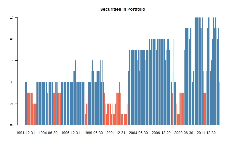
Figure 1 shows the total number of securities at any given time in the OP portfolio. Notice the red bars represent those times that there were less than 4 securities in the portfolio in which case the optimization was not run and equal weighting given to each security.
Results and Discussion
| 1994-2013 | OPalt | OP | EQ | S&P500 | 2000-2013 | OPalt | OP | EQ | S&P500 | |
|---|---|---|---|---|---|---|---|---|---|---|
| CAGR | 8.94 | 11.16 | 10.34 | 6.52 | CAGR | 8.45 | 9.89 | 8.21 | 0.24 | |
| Vol | 8.43 | 10.92 | 11.65 | 19.5 | Vol | 9.19 | 11.88 | 12.82 | 21.18 | |
| Sharpe | 0.71 | 0.76 | 0.65 | 0.27 | Sharpe | 0.7 | 0.68 | 0.52 | 0.02 | |
| LW p-value | 0.113 | 0.154 | LW p-value | 0.03 | 0.078 | |||||
| BestM | 6.63 | 9.82 | 9.82 | 10.5 | BestM | 6.3 | 9.04 | 6.96 | 10.5 | |
| WorstM | -6.91 | -10.54 | -10.54 | -19.14 | WorstM | -5.89 | -8.84 | -7.01 | -19.14 | |
| UpM | 69.4 | 68.53 | 63.36 | 63.09 | UpM | 67.5 | 67.5 | 62.5 | 59.01 | |
| DnM | 30.6 | 31.47 | 36.64 | 36.91 | DnM | 32.5 | 32.5 | 37.5 | 40.99 | |
| MaxDraw | 14.5 | 19.04 | 19.04 | 59.65 | MaxDraw | 14.5 | 18.65 | 18.24 | 59.65 |
| 2003-2013 | OPalt | OP | EQ | S&P500 | 2010-2013 | OPalt | OP | EQ | S&P500 | |
|---|---|---|---|---|---|---|---|---|---|---|
| CAGR | 11.49 | 13.93 | 12.21 | 5.79 | CAGR | 7.36 | 8.23 | 4.19 | 11.77 | |
| Vol | 9.83 | 12.49 | 13.68 | 20.52 | Vol | 7.39 | 8.92 | 11.93 | 17.81 | |
| Sharpe | 0.99 | 0.98 | 0.79 | 0.3 | Sharpe | 0.99 | 0.92 | 0.4 | 0.71 | |
| LW p-value | 0.065 | 0.1 | LW p-value | 0.054 | 0.098 | |||||
| BestM | 6.3 | 9.04 | 6.96 | 10.5 | BestM | 3.88 | 5.76 | 6.1 | 10.5 | |
| WorstM | -5.89 | -8.84 | -7.01 | -19.14 | WorstM | -5.89 | -8.84 | -7.01 | -8.37 | |
| UpM | 70.97 | 70.97 | 64.52 | 64.8 | UpM | 67.5 | 67.5 | 57.5 | 63.41 | |
| DnM | 29.03 | 29.03 | 35.48 | 35.2 | DnM | 32.5 | 32.5 | 42.5 | 36.59 | |
| MaxDraw | 14.5 | 18.65 | 18.24 | 59.65 | MaxDraw | 10.13 | 14.83 | 18.24 | 20.03 |
Tables 1 and 2 present the results for various subperiods of the 2 optimal portfolios, the equal weighted portfolio and the S&P 500 index (as captured by the VFINX fund). I use subperiod analysis since half of the securities in the universe only start in the early to mid 2000s, which means that the 1990-2000 period is contaminated with a small number of assets and hence more likely to have equal weights (when the number of signals is less than 4 the model allocates equally to each). The results provide for a very clear picture of the incremental value of each portfolio. The OP and EW portfolios, over the whole sample appear to have the same drawdowns. This is likely related to the fact that both portfolios have the same signal generating mechanism which somewhat lags the turning points and is based on monthly data (so that daily P&L accounting is likely to reveal larger intra-month fluctuations). The OPalt portfolio on the other hand, which makes use of information from the DGP and optimal weight vector has lower drawdowns which indicates that there is value in making use of information from this model beyond what the signals provide for timing purposes. The Sharpe ratios for the optimal portfolios are higher than that of the equal weighted portfolio in all subperiods, but significantly different at the 10% level only the period after 2000 (the ‘LW p-value’ row contains the p-values from the test of Ledoit and Wolf (2008) of the optimal portfolio against the equal weighted portfolio under the null hypothesis that their Sharpe ratio differences are zero), again for the reasons hypothesized earlier. Overall, one may cautiously conclude from this small example that there is value in adopting a disciplined quantitative approach to the allocation of capital beyond the naive 1/N approach.
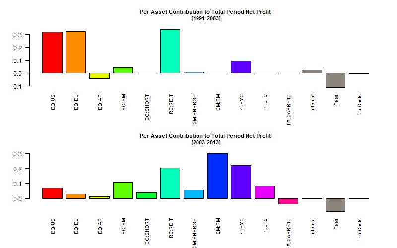
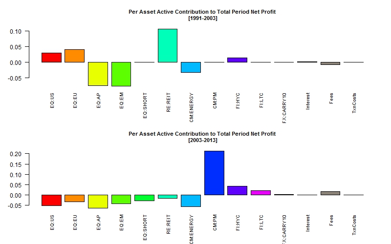
Figure 2a gives the contribution to P&L of each security over 2 subperiods, whilst Figure 2b gives the active contribution (over the equal weighted portfolio) of each security to P&L, which gives some additional insight to where the bets where concentrated.
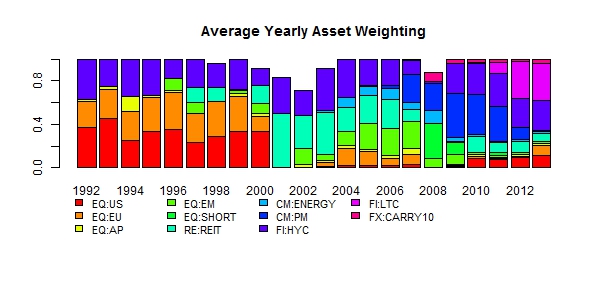
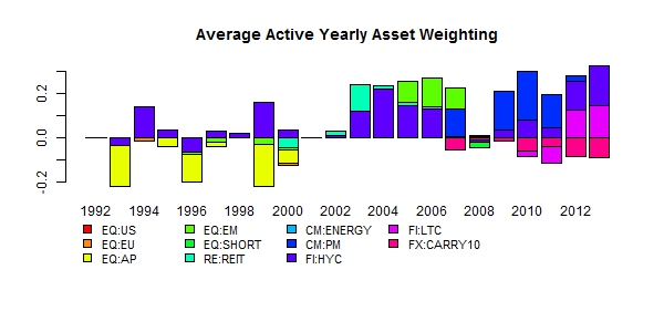
Figure 3a shows the average yearly allocation per security of the optimal portfolio, whilst Figure 3b the active allocation (over the equal weighted portfolio). The figures show a clear difference between the optimal and equal allocation methods, with the former having made positive active bets on Gold and High Yield Corporates over the entire period, and underweighted Asia Pacific Equities in the 1990s.
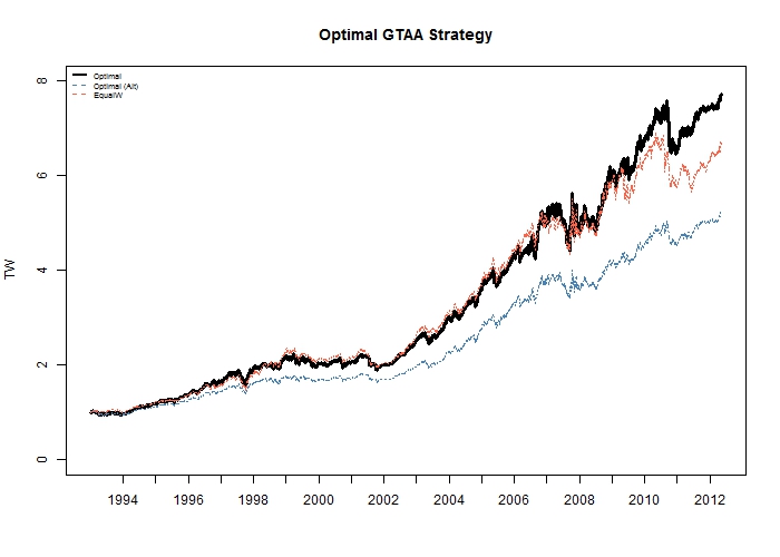
Finally, Figure 4 provides the evolution of Terminal Wealth for the 3 portfolios, though this is always somewhat less informative than the subperiod analysis since it always depends on the starting point and will not usually be a good indicator of the average risk-return profile, as can be deduced from the OPalt portfolio which has the lowest Terminal Wealth but the highest Sharpe Ratio and lowest drawdowns.
Conclusion
There is really no substitute for a disciplined approach to the modelling of security dynamics and stochastic programming to obtain the optimal weights. Even when there is not enough data, it is certainly possible to map the data available to either a set of higher frequency factors or closely related prospects with more data. This article provided for a very simple example of what is possible. Interesting extensions to the approach adopted might include:
- A more sophisticated signal generating mechanism, taking into account explanatory variables (not just looking at the price trend) for turning point or directional analysis.
- More advanced money management overlay to limit intra-month losses. The blotter wrapper function allows for this and a simple example is included (though not used) in the code. To my knowledge it remains an open question whether stop losses add or subtract value, and it is my experience that including them within a strategy for intra-month risk reduction should be done with caution.
- No short sale constraint. Technically, there is no reason not to remove the constraint, but the realistic modelling of this is more complicated because of the need to track margin etc. The blotter wrapper is not yet setup to deal with this case.
Code
There are 5 files in the zip (unstarched_code). Place them in an empty directory which you will designate as your working directory in R (‘setwd’). The main file which you will need to run is the ‘unstarched_script_run.R’ file. Be patient, it takes some time to complete, mainly because of the portfolio trades/accounting, the progress of which will be displayed on screen. I estimate about 60 minutes to complete.
References
Demey, P., Maillard, S., & Roncalli, T. (2010). Risk-based indexation. Available at SSRN 1582998.
DeMiguel, V., Garlappi, L., & Uppal, R. (2009). Optimal versus naive diversification: How inefficient is the 1/N portfolio strategy?. Review of Financial Studies, 22(5), 1915-1953.
Faber, M. T. (2007). A quantitative approach to tactical asset allocation. Journal of Wealth Management.
Gibbons, M. R., Ross, S. A., & Shanken, J. (1989). A test of the efficiency of a given portfolio. Econometrica: Journal of the Econometric Society, 1121-1152.
Grinold, R. C. (1992). Are Benchmark Portfolios Efficient?. The Journal of Portfolio Management, 19(1), 34-40.
Kritzman, M., Page, S., & Turkington, D. (2010). In defense of optimization: the fallacy of 1/N. Financial Analysts Journal, 66(2), 31.
Ledoit, O., & Wolf, M. (2008). Robust performance hypothesis testing with the Sharpe ratio. Journal of Empirical Finance, 15(5), 850-859.
extremely well done and beautiful. great job.
Thanks!
Great post; It seems however, that the Ledoit Wolf test used here is extremely powerful–almost too powerful. Cherry picking an example, the comparison for 2003-2013, a 10 year period, over which OPalt and EQN have Sharpe ratios of 0.99 and 0.79, the test almost rejects at the 0.05 level. I realize this is a paired test, which should be more powerful than e.g. a normal approximation, but the standard error for Sharpe over a 10 year time frame should be around 0.3, meaning that 0.79 and 0.99 are statistically equivalent. Am I missing something, or is the test really that powerful?
I think the moment you accept that there is some departure from the Normal and i.i.d assumption, then you cannot scale by sqrt of time. In particular, the presence of positive (negative) serial correlation in the returns will inflate (deflate) the ‘true’ Sharpe ratio (Andrew Lo FAJ 2002 paper). The test uses a studendized circular block bootstrap procedure which also requires calibration (the calibration found the optimal block length to be 10). IMHO i think that the difference in the ratios will depend on the properties of the returns and in that respect it is quite powerful in picking those up rather than making the standard normal approximation assumptions.
As an aside, have you thought of including the test in your SharpeR package (it could also do with some Rcpp recoding for speed)?
I am not sure Normality is required for sqrt time scaling, but violation of i.i.d. would certainly be a problem. I do not think autocorrelation is going to be such a huge issue, however: the geometric bias in Sharpe ratio is on the order of the autocorrelation when the latter is small (the standard t-stat correction), and I expect autocorrelation in stock returns to have been ‘arbed out’ to below 0.05 or so. YMMV on that.
You did read my mind regarding implementing the L-W test; I have been having problems with the Leung-Wong/Wright-Yam-Yung test where it appears to reject equality of Sharpe for ‘uninteresting reasons’, and was looking for an alternative. Have you stress tested the L-W test and found that it maintains nominal type I rate?
Indeed, normality is not strictly required for scaling unless dealing with quantiles.
I’m not sure as to the other points. Even though the OP and OPalt portfolios have very close Sharpe ratios during some of the subperiods, and indeed are almost similar as models except for improved timing in the latter, their p-values are somewhat different reflecting this subtle difference in their return distributions. I do think that this is quite a powerful test…but have not stress tested it. There are a couple of tables in the original paper for its performance under alternative DGPs.