The last model added to the rugarch package dealt with the modelling of intraday volatility using a multiplicative component GARCH model. The newest addition is the realized GARCH model of Hansen, Huang and Shek (2012) (henceforth HHS2012) which relates the realized volatility measure to the latent volatility using a flexible representation with asymmetric dynamics. This short article discusses the model, its implementation in rugarch and a short empirical application.
The Model
The realized GARCH (realGARCH) model of HHS2012 provides for an excellent framework for the joint modelling of returns and realized measures of volatility. Unlike the naive augmentation of GARCH processes by a realized measures, the realGARCH model relates the observed realized measure to the latent volatility via a measurement equation, which also includes asymmetric reaction to shocks, making for a very flexible and rich representation. Formally, let:
\[ \begin{gathered}
{y_t} = {\mu _t} + {\sigma _t}{z_t},{\text{ }}{z_t} \sim i.i.d\left( {0,1} \right) \\
\log \sigma _t^2 = \omega + \sum\limits_{i = 1}^q {{\alpha _i}\log {r_{t – i}} + \sum\limits_{i = 1}^p {{\beta _i}\log \sigma _{t – i}^2} } \\
\log r_t = \xi + \delta \log \sigma _t^2 + \tau \left( {{z_t}} \right) + {u_t},{\text{ }}{u_t} \sim N\left( {0,\lambda } \right) \\
\end{gathered}
\]
where we have defined the dynamics for the returns (\( y_t \)), the log of the conditional variance (\( \sigma^2_t \)) and the log of the realized measure (\( r_t \)). Note that the notation varies slightly from that of HHS2012, and the rugarch vignette contains a footnote of the differences. The asymmetric reaction to shocks comes via the \( \tau\left(.\right) \) function which is based on the Hermite polynomials and truncated at the second level to give a simple quadratic form:
\[ \tau\left(z_t\right) = \eta_1z_t + \eta_2\left(z^2_t-1\right)
\]
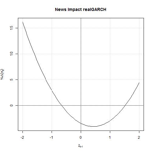
which has the very convenient property that \( E\tau\left(z_t\right)=0 \). The function also forms the basis for the creation of a type of news impact curve \( \nu \left( z \right) \), defined as:
\[ \begin{gathered}
\nu \left( z \right) = E\left[ {\log {\sigma _t}\left| {{z_{t – 1}} = z} \right.} \right] – E\left[ {\log {\sigma _t}} \right] = \delta \tau \left( z \right) \\
\end{gathered}
\]
so that \( 100\times\nu\left(z\right) \) is the percent change in volatility as a function of the standardized innovations.
A key feature of this model is that it preserves the ARMA structure which characterize many standard GARCH models and adapted here from Proposition 1 of the HHS2012 paper:
\[ \begin{gathered}
\log \sigma _t^2 = {\mu _\sigma } + \sum\limits_{i = 1}^{p \vee q} {\left( {\delta {\alpha _i} + {\beta _i}} \right)\log \sigma _{t – 1}^2 + } \sum\limits_{j = 1}^q {{\alpha _j}{w_{t – j}}} \\
\log {r_t} = {\mu _r} + \sum\limits_{i = 1}^{p \vee q} {\left( {\delta {\alpha _i} + {\beta _i}} \right)\log {r_{t – 1}} + {w_t}} – \sum\limits_{j = 1}^{p \vee q} {{\beta _j}{w_{t – j}}} \\
{\mu _\sigma } = \omega + \xi \sum\limits_{i = 1}^q {{\alpha _i}} ,{\mu _r} = \delta \omega + \left( {1 – \sum\limits_{i = 1}^p {{\beta _i}} } \right)\xi \\
\end{gathered}
\]
where \( w_t=\tau\left(z_t\right)+u_t \), \( {\mu _\sigma } = \omega + \xi \sum\limits_{i = 1}^q {{\alpha _i}} \) and \( {\mu _r} = \delta \omega + \left( {1 – \sum\limits_{i = 1}^p {{\beta _i}} } \right)\xi \), and the convention \( {\beta _i} = {\alpha _j} = 0 \) for \( i>p \) and \( j\lt p \). It is therefore a simple matter to show that the persistence \(\hat P\) of the process is given by:
\[
\hat P = \sum\limits_{i = 1}^p {{\beta _i} + } \delta \sum\limits_{i = 1}^q {{\alpha _i}}
\]
while the unconditional (long-run) variance may be written as:
\[
{\hat \sigma ^2} = \frac{{\omega + \xi \sum\limits_{i = 1}^q {{\alpha _i}} }}
{{1 – \hat P}}
\]
Demonstration: Estimation
For the demonstration, I will use the SPY dataset which accompanied the paper of HHS2012 including the realized volatility based on the realized kernel (parzen) method of Barndorff-Nielsen et al (2008) (this dataset is now included in rugarch as of version 1.3-0). In general, the highfrequency package can be used on intraday data to generate any number of realized volatility measures (and is currently the only package AFAIK that provides this functionality in R).
library(rugarch) require(xts) data(spyreal) spec = ugarchspec(mean.model = list(armaOrder = c(0, 0), include.mean = FALSE), variance.model = list(model = 'realGARCH', garchOrder = c(2, 1))) setbounds(spec)<-list(alpha2=c(-1,1)) fit = ugarchfit(spec, spyreal[, 1] * 100, solver = 'hybrid', realizedVol = spyreal[,2] * 100)Notice how the additional realized measure is passed via the realizedVol argument which must be an xts object with matching index as the returns data. Also note the use of the hybrid solver which is the recommended method for solving this type of model.
I’m going to compare the results with those of HHS2012:
cf = coef(fit) se = fit@fit$matcoef[, 2] names(se) = names(cf) # HHS2012 divide the period into in-(T=1492) and out- of sample, even though they are estimating the model using the entire dataset (T=1659)...no comment. benchmark.LL = c('logL' = -2388.75, 'pLogL' = -1710.34) benchmark.pars = c('logh0' = -0.289213754, 'omega' = 0.041246175, 'alpha1' = 0.450676773, 'alpha2' = -0.176042911, 'beta1' = 0.701210369, 'xi' = -0.179994885, 'delta' = 1.037491982, 'eta1' = -0.067809509, 'eta2' = 0.07015778, 'lambda' = sqrt(0.145369801)) benchmark.se = c('logh0' = 0.278787604, 'omega' = 0.015515016, 'alpha1' = 0.038027571, 'alpha2' = 0.06335417, 'beta1' = 0.055974942, 'xi' = 0.043611245, 'delta' = 0.057726499, 'eta1' = 0.010309694, 'eta2' = 0.006620828, 'lambda' = 0.00594321) # rugarch does not estimate h0, instead uses either mean(residuals^2), else a choice of variance targeting with options rugarch.LL = c('logL' = sum(-fit@fit$log.likelihoods[1:1492]), 'pLogL' = sum(-fit@fit$partial.log.likelihoods[1:1492])) rugarch.pars = c('logh0' = NA, 'omega' = cf['omega'], 'alpha1' = cf['alpha1'], 'alpha2' = cf['alpha2'], 'beta1' = cf['beta1'], 'xi' = cf['xi'], 'delta' = cf['delta'], 'eta1' = cf['eta11'], 'eta2' = cf['eta21'], 'lambda' = cf['lambda']) rugarch.se = c('logh0' = NA, 'omega' = se['omega'], 'alpha1' = se['alpha1'], 'alpha2' = se['alpha2'], 'beta1' = se['beta1'], 'xi' = se['xi'], 'delta' = se['delta'], 'eta1' = se['eta11'], 'eta2' = se['eta21'], 'lambda' = se['lambda']) names(rugarch.pars) = names(rugarch.se) = c('logh0', 'omega', 'alpha1', 'alpha2', 'beta1', 'xi', 'delta', 'eta1', 'eta2', 'lambda') parsdf = cbind(benchmark.pars, rugarch.pars, benchmark.pars - rugarch.pars) sedf = cbind(benchmark.se, rugarch.se, benchmark.se - rugarch.se) LRE.vars = -log(abs(rugarch.pars - benchmark.pars)/abs(benchmark.pars), base = 10) LRE.se = -log(abs(rugarch.se - benchmark.se)/abs(benchmark.se), base = 10) test = cbind(LRE.vars, LRE.se) tmp1 = t(cbind(rugarch = rugarch.pars, benchmark = benchmark.pars)) tmp2 = t(cbind(rugarch = rugarch.se, benchmark = benchmark.se)) # print the results: ## parameters: ## logh0 omega alpha1 alpha2 beta1 xi delta eta1 eta2 lambda ## rugarch NA 0.0451 0.4766 -0.2027 0.7050 -0.1898 1.027 -0.0616 0.0718 0.3815 ## benchmark -0.2892 0.0412 0.4507 -0.1760 0.7012 -0.1800 1.038 -0.0678 0.0702 0.3813 ## ## standard errors: ## logh0 omega alpha1 alpha2 beta1 xi delta eta1 eta2 lambda ## rugarch NA 0.0137 0.0289 0.0450 0.0381 0.0390 0.0403 0.0097 0.0062 0.0066 ## benchmark 0.2788 0.0155 0.0380 0.0634 0.0560 0.0436 0.0577 0.0103 0.0066 0.0059 ## ## Log Relative Error Test: ## logh0 omega alpha1 alpha2 beta1 xi delta eta1 eta2 lambda ## LRE.vars NA 1.0293 1.2408 0.8191 2.2627 1.2640 2.012 1.041 1.623 3.1413 ## LRE.se NA 0.9355 0.6212 0.5374 0.4947 0.9733 0.519 1.204 1.208 0.9435The results are pretty close, and all parameters are found to be highly significant. Note that unlike HHS2012, rugarch does not include \( h_0 \) in the parameter estimation set but instead, like the other models, estimates it based on the filtered squared residuals. Finally, we reproduce the news impact curve from their paper:
ni = newsimpact(fit, z = seq(-2, 2, length.out = 100)) plot(ni$zx, (ni$zy), ylab = ni$yexpr, xlab = ni$xexpr, type = 'l', main = 'News Impact realGARCH') abline(v = 0) abline(h = 0) grid()
The interested reader should read the HHS2012 paper which has some very good insights. In particular, the coefficient on the log conditional variance in the measurement equation (\(\delta\)) provides interesting insights depending on whether open-close or close-close returns are used.Demonstration: Forecasting
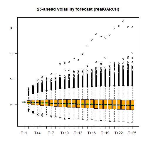
In rugarch, it is possible to create both rolling 1-ahead forecasts (assuming the out.sample option was used in the estimation) and long-run n-ahead forecasts, and combinations of both. In the realGARCH model, n.ahead>1 forecasts contain uncertainty because \( u_t \) is not known. As such, simulation methods are used and the ugarchforecast routine takes on additional arguments related to this. These are n.sim for the number of random samples to use per period for the generation of the discrete time density of the forecast variance (and also the realized volatility), and returnDistribution (logical) indicates whether to include these estimates of the density in the returned object. Whatever the case, the point estimate is always returned and based on the mean of the sampled values.
The first example below demonstrates the equivalence of the ugarchfilter and ugarchforecast (using either a uGARCHfit or uGARCHspec objects) methods.
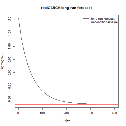
fit = ugarchfit(spec, spyreal[, 1] * 100, out.sample = 25, solver = 'hybrid', realizedVol = spyreal[, 2] * 100) specf = spec setfixed(specf) < - as.list(coef(fit)) filt = ugarchfilter(specf, data = spyreal[, 1] * 100, n.old = nrow(spyreal) - 25, realizedVol = spyreal[, 2] * 100) forc1 = ugarchforecast(fit, n.ahead = 1, n.roll = 25) # forecast from spec forc2 = ugarchforecast(specf, n.ahead = 1, n.roll = 25, data = spyreal[, 1] * 100, out.sample = 25, realizedVol = spyreal[, 2] * 100) filts = tail(sigma(filt), 25) colnames(filts) = 'filter' forcs1 = xts(sigma(forc1)[1, ], move(as.Date(names(sigma(forc1)[1, ])), by = 1)) forcs2 = xts(sigma(forc2)[1, ], move(as.Date(names(sigma(forc2)[1, ])), by = 1)) colnames(forcs1) = 'fit2forecast' colnames(forcs2) = 'spec2forecast' ftest = cbind(filts, forcs1, forcs2) # last forecast is completely out of sample, so not available from the # filter method (which filters given T-1) print(round(ftest, 5)) ## filter fit2forecast spec2forecast ## 2008-07-28 1.1065 1.1065 1.1065 ## 2008-07-29 1.0131 1.0131 1.0131 ## 2008-07-30 0.9885 0.9885 0.9885 ## 2008-07-31 1.0828 1.0828 1.0828 ## 2008-08-01 1.0685 1.0685 1.0685 ## 2008-08-04 1.1434 1.1434 1.1434 ## 2008-08-05 1.0460 1.0460 1.0460 ## 2008-08-06 1.0351 1.0351 1.0351 ## 2008-08-07 0.9206 0.9206 0.9206 ## 2008-08-08 0.9933 0.9933 0.9933 ## 2008-08-11 1.0083 1.0083 1.0083 ## 2008-08-12 0.9368 0.9368 0.9368 ## 2008-08-13 0.9564 0.9564 0.9564 ## 2008-08-14 1.0243 1.0243 1.0243 ## 2008-08-15 0.9903 0.9903 0.9903 ## 2008-08-18 0.9432 0.9432 0.9432 ## 2008-08-19 0.9751 0.9751 0.9751 ## 2008-08-20 0.9453 0.9453 0.9453 ## 2008-08-21 1.0326 1.0326 1.0326 ## 2008-08-22 0.9930 0.9930 0.9930 ## 2008-08-25 0.8638 0.8638 0.8638 ## 2008-08-26 0.9082 0.9082 0.9082 ## 2008-08-27 0.9154 0.9154 0.9154 ## 2008-08-28 0.8658 0.8658 0.8658 ## 2008-08-29 0.8235 0.8235 0.8235 ## 2008-09-01 NA 0.8103 0.8103The advantage of being able to call the ugarchforecast method with a uGARCHspec object (with fixed pars) should be obvious. Anytime we have new data arriving, we can simply augment the old data and create new forecasts without having to re-estimate the model (unless we wish to update the parameter set). In the next example, a long-horizon forecast is created an compared to the unconditional value:
set.seed(55) forc3 = ugarchforecast(fit, n.ahead = 400, n.sim = 5000) plot(sigma(forc3), type = 'l', main = 'realGARCH long-run forecast') abline(h = sqrt(uncvariance(fit)), col = 2) legend('topright', c('long-run forecast', 'unconditional value'), col = 1:2, lty = c(1, 1), bty = 'n')The final example shows how the forecast density is extracted from the forecasted object. This is an array of dimensions (n.ahead x n.sim x n.roll+1).
set.seed(55) forc4 = ugarchforecast(fit, n.ahead = 25, n.sim = 10000) # dim(forc4@forecast$sigmaDF) sigmaDF = forc4@forecast$sigmaDF meansig = sqrt(exp(rowMeans(log(sigmaDF[, , 1]^2)))) boxplot(t(sigmaDF[, , 1]), main = '25-ahead volatility forecast (realGARCH)', col = 'orange') points(as.numeric(meansig), col = 'green') # note that for the 1-ahead there is no uncertainty (unless we were doing this Bayes-style so that parameter uncertainty would have an impact).Demonstration: Simulation
There are 2 ways to simulate from GARCH models in the rugarch package: either directly from an estimated object (uGARCHfit class) or from a GARCH spec (uGARCHspec with fixed parameters), similarly to the ugarchforecast method. However, instead of having a single dispatch method, there is ugarchsim (for the uGARCHfit class) and ugarchpath (for the uGARCHspec class). In the example that follows I show how to generate equivalent values from the two methods:
spec = ugarchspec(mean.model = list(armaOrder = c(1, 1), include.mean = TRUE), variance.model = list(model = 'realGARCH', garchOrder = c(1, 1))) fit = ugarchfit(spec, spyreal[, 1] * 100, out.sample = 25, solver = 'hybrid', realizedVol = spyreal[, 2] * 100) specf = spec setfixed(specf) < - as.list(coef(fit)) T = nrow(spyreal) - 25 sim1 = ugarchsim(fit, n.sim = 1000, m.sim = 1, n.start = 0, startMethod = 'sample', rseed = 12) sim2 = ugarchsim(fit, n.sim = 1000, m.sim = 1, n.start = 0, startMethod = 'sample', rseed = 12, prereturns = as.numeric(tail(spyreal[1:T, 1] * 100, 1)), presigma = as.numeric(tail(sigma(fit), 1)), preresiduals = as.numeric(tail(residuals(fit), 1)), prerealized = as.numeric(tail(spyreal[1:T, 2] * 100, 1))) sim3 = ugarchpath(specf, n.sim = 1000, m.sim = 1, n.start = 0, rseed = 12, prereturns = as.numeric(tail(spyreal[1:T, 1] * 100, 1)), presigma = as.numeric(tail(sigma(fit), 1)), preresiduals = as.numeric(tail(residuals(fit), 1)), prerealized = as.numeric(tail(spyreal[1:T, 2] * 100, 1))) print(cbind(head(sigma(sim1)), head(sigma(sim2)), head(sigma(sim3)))) ## [,1] [,2] [,3] ## T+1 1.0735 1.0735 1.0735 ## T+2 0.9836 0.9836 0.9836 ## T+3 1.1091 1.1091 1.1091 ## T+4 1.0306 1.0306 1.0306 ## T+5 0.9609 0.9609 0.9609 ## T+6 0.8771 0.8771 0.8771Again, it should be obvious what the applications are for ugarchpath in a live environment.
Application: Rolling Forecasts and Value at Risk
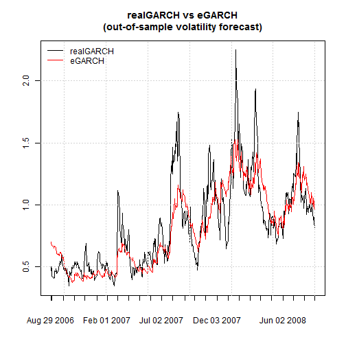
The final part of this article provides a small empirical application comparing the realGARCH and eGARCH models for risk management.
library(parallel) cl = makePSOCKcluster(5) spec1 = ugarchspec(mean.model = list(armaOrder = c(1, 1), include.mean = TRUE), variance.model = list(model = 'realGARCH', garchOrder = c(1, 1))) spec2 = ugarchspec(mean.model = list(armaOrder = c(1, 1), include.mean = TRUE), variance.model = list(model = 'eGARCH', garchOrder = c(1, 1))) roll1 = ugarchroll(spec1, spyreal[, 1] * 100, forecast.length = 500, solver = 'hybrid', refit.every = 25, refit.window = 'recursive', realizedVol = spyreal[, 2] * 100, cluster = cl) roll2 = ugarchroll(spec2, spyreal[, 1] * 100, forecast.length = 500, refit.every = 25, refit.window = 'recursive', cluster = cl) report(roll1) ## VaR Backtest Report ## =========================================== ## Model: realGARCH-norm ## Backtest Length: 500 ## Data: ## ## ========================================== ## alpha: 1% ## Expected Exceed: 5 ## Actual VaR Exceed: 10 ## Actual %: 2% ## ## Unconditional Coverage (Kupiec) ## Null-Hypothesis: Correct Exceedances ## LR.uc Statistic: 3.914 ## LR.uc Critical: 3.841 ## LR.uc p-value: 0.048 ## Reject Null: YES ## ## Conditional Coverage (Christoffersen) ## Null-Hypothesis: Correct Exceedances and ## Independence of Failures ## LR.cc Statistic: 4.323 ## LR.cc Critical: 5.991 ## LR.cc p-value: 0.115 ## Reject Null: NO ## ## report(roll2) ## VaR Backtest Report ## =========================================== ## Model: eGARCH-norm ## Backtest Length: 500 ## Data: ## ## ========================================== ## alpha: 1% ## Expected Exceed: 5 ## Actual VaR Exceed: 16 ## Actual %: 3.2% ## ## Unconditional Coverage (Kupiec) ## Null-Hypothesis: Correct Exceedances ## LR.uc Statistic: 15.467 ## LR.uc Critical: 3.841 ## LR.uc p-value: 0 ## Reject Null: YES ## ## Conditional Coverage (Christoffersen) ## Null-Hypothesis: Correct Exceedances and ## Independence of Failures ## LR.cc Statistic: 16.527 ## LR.cc Critical: 5.991 ## LR.cc p-value: 0 ## Reject Null: YES ## ## plot(as.xts(as.data.frame(roll1)[, 'Sigma', drop = FALSE]), main = 'realGARCH vs eGARCH\n(out-of-sample volatility forecast)', auto.grid = FALSE, minor.ticks = FALSE) lines(as.xts(as.data.frame(roll2)[, 'Sigma', drop = FALSE]), col = 2) legend('topleft', c('realGARCH', 'eGARCH'), col = 1:2, lty = c(1, 1), bty = 'n') grid()Peachy!
Conclusion
As widely reported in various applications and papers, there is no denying the value of including realized measures in the modelling process, particularly when done in a flexible and rich framework as offered by the realized GARCH model.
Happy 2014.
References
Barndorff-Nielsen, O. E., Hansen, P. R., Lunde, A., & Shephard, N. (2008). Designing realized kernels to measure the ex post variation of equity prices in the presence of noise. Econometrica, 76(6), 1481-1536.
Hansen, P. R., Huang, Z., & Shek, H. H. (2012). Realized GARCH: a joint model for returns and realized measures of volatility. Journal of Applied Econometrics, 27(6), 877-906.


