What is risk parity (RP)?
Simply put, it is a method of allocating equal risk shares to each asset in the portfolio. In more traditional allocation schemes, equity, being the riskiest asset (and hence providing the highest reward), has typically received the lion’s share. With RP, equalization of risk contribution means that equity and other similarly risky assets receive a reduced allocation and low risk assets such as government bonds an increased allocation. As a result, in order to achieve ‘equity-like’ total returns, leverage has typically been used in this context, possibly using a target risk level. Under certain circumstances, namely when all assets have the same risk-to-reward ratios, the RP allocation is equivalent to the tangent portfolio. In the case where only the risks are equal, then the RP allocation is generally equivalent to the equal weight (1/n) portfolio, whilst it coincides with the minimum risk portfolio when cross diversification is highest (though that may be a tricky concept to describe when going beyond the mean-variance paradigm).
Of course, like all portfolio problems, we are speaking of our expectations of future risk. And this is one of the key benefits, argue the proponents of RP, since variance is much more stable and easier to forecast than the returns. Therefore, lying somewhere between the minimum risk and optimal risk portfolios, making use of only the ‘risk’ rather than the reward in the calculation, and backed up by an apparently stellar performance resulting from the recent decline in US Treasury rates, one might wonder why portfolio allocation is still taught at university.
In this author’s opinion, RP is not a proper model of asset allocation, does not contain that key ingredient called an active forecast which is after all what managers are rewarded for producing, and is likely to create complacency because of its oversimplified approach to the problem of forecast uncertainty. In this article I provide 2 applications based on different datasets with different characteristics in order to highlight some issues with the RP approach. I examine different risk\(^1\) measures, within a simple parametric DGP framework for generating forecasts, and find that even with such a simple approach RP cannot outperform the optimal risk-reward strategy or even the minimum risk strategy in a well diversified universe.
Initial Formalities
Formally, consider the marginal contribution to risk (MCR) of each asset (\(i\) of \(n\)) given a risk measure \( \rho\left(x\right) \):
\[
MC{R_i} = \frac{{\partial \rho \left( x \right)}}{{\partial {x_i}}}
\]
which when multiplied by the asset’s share and summed leads to the total portfolio risk (TR):
\[
TR = \sum\limits_{\forall i} {{x_i}MC{R_i}}
\]
One way to solve the general RP problem was already suggested by Maillard, Roncalli and Teïletche (2010) as a squared error minimization type problem which can be easily solved with an SQP solver:
\[
\begin{gathered}
\mathop {{\text{min}}}\limits_{\mathbf{x}} {\text{ }}\sum\limits_{j = 1}^n {\sum\limits_{i = 1}^n {{{\left( {{x_i}MC{R_i} – {x_j}MC{R_j}} \right)}^2}} }\\
s.t. \\
\sum\limits_{\forall i} {{x_i} = b} \\
{\mathbf{x}} \geqslant 0 \\
\end{gathered}
\]
where \( b \) is the budget constraint. It should be clear that MCR is just the gradient of the risk function. Since all NLP risk functions in the parma package have analytic gradients (see the vignette for details), then the extension of RP to other measures beyond variance is quite trivial. For the case of variance, a fast algorithm using Newton’s method proposed by Chaves, Hsu and Shakernia (2012) is also available and tests conducted indicate that it is upto 100x faster than the equivalent SQP optimization (though we are already talking about tenths of a second anyway).
Set 1: Low Diversity Universe
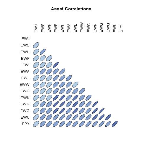
The dataset consists of weekly (Friday) returns of international equity ETFs for the period November-2000 to December 2013. It is a highly correlated dataset with low diversification possibilities in a long-only setup. As such, it serves to illustrate the similarities between the equally weighted and RP portfolios.
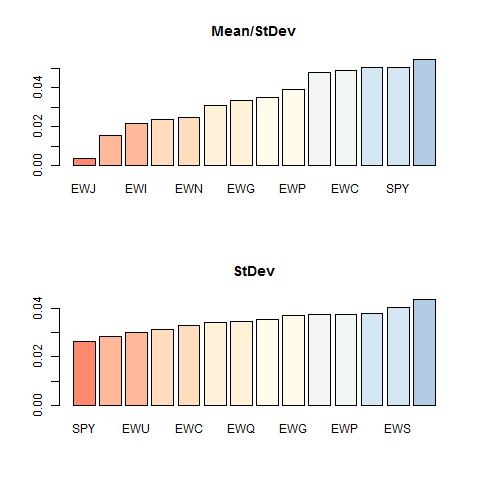
Figure 1 aptly illustrates the very high correlation of the dataset whilst Figure 2 provides an indication of the risk and risk-return profile of the dataset, though one should bear in mind that this is for the entire period and does not necessarily reflect the situation at any particular point in time.
The backtest uses a static normal copula to model the covariance, with first stage AR(1)-GARCH(1,1)-JSU dynamics. The choice of a static rather than dynamic correlation model was motivated by the size of the dataset which is quite small, whilst for the conditional first stage GARCH dynamics the JSU distribution was used to account for univariate higher moments. Finally, and again motivated by the size of the dataset, an empirical transformation was used (see Genest, Ghoudi and Rivest (1995) and the rmgarch vignette for more details). At each time T (a Friday), data from 1:T was used (hence an expanding window choice) for the modelling, after which the T+1 simulated forecast density (the scenario) was generated for use in the optimization model. For the Mean-Variance model, the covariance of the simulated T+1 forecast density was used, whilst for all other risk measures the actual scenario was used in the optimization.
Three models were evaluated: the minimum risk (MR), risk parity (RP) and optimal risk-reward (OPT) using fractional programming. Within those models, four risk measures were evaluated: mean-variance (EV), mean absolute deviation (MAD) and lower partial moments of orders 2 and 4 (LPM2 and LPM4) representing different aversions to below threshold losses\( ^{2} \).
The weights generated by each model where then used to buy the underlying assets at the close of the day after (i.e. Monday) and held until the following re-formation period (i.e. the next Monday). In this way, there was no contemporaneous signal-portfolio formation bias, which may be significant for weekly and higher frequency models. Trading costs were not included nor was price impact and other related costs.
Table 1 provides a summary of the results (using the equal weight as the benchmark), with the key points being:
- Among the allocation models, there is a negligible difference between the different risk measures. This may represent the frequency of the dataset and/or the DGP used (normal copula).
- The RP and equal weight portfolios appear very close, as might be expected from the very close ex-ante variance of the assets and high correlation.
- The MR portfolio shows dismal performance, and this is in line with the little diversification potential of this dataset.
- The OPT portfolio appears superior to the RP model on all measures. Statistical significance of this statement was not checked, and with the exception of the Sharpe ratio one is challenged to do so for a large number of measures even on moderately sized datasets.
Table-1
| SET-1 | RP[EV] | RP[MAD] | RP[LPM2] | RP[LPM4] | MR[EV] | MR[MAD] | MR[LPM2] | MR[LPM4] | OPT[EV] | OPT[MAD] | OPT[LPM2] | OPT[LPM4] | EW |
|---|---|---|---|---|---|---|---|---|---|---|---|---|---|
| CAGR | 7.04 | 6.99 | 6.97 | 7.01 | 3.44 | 2.35 | 3.34 | 4.60 | 10.22 | 10.00 | 9.91 | 9.70 | 7.73 |
| SD | 32.99 | 32.98 | 32.95 | 32.94 | 28.15 | 28.14 | 27.95 | 28.01 | 34.89 | 34.82 | 34.83 | 34.81 | 34.03 |
| Up | 54.17 | 54.03 | 53.88 | 54.03 | 55.34 | 54.90 | 54.90 | 55.64 | 54.61 | 54.90 | 55.05 | 54.76 | 54.32 |
| MaxDrawdown | 77.51 | 77.52 | 77.46 | 77.39 | 74.54 | 75.49 | 74.44 | 73.35 | 71.37 | 71.20 | 71.08 | 70.77 | 77.74 |
| CAPM[alpha] | -0.62 | -0.67 | -0.69 | -0.65 | -3.49 | -4.53 | -3.57 | -2.36 | 2.98 | 2.79 | 2.68 | 2.49 | 0.00 |
| CAPM[beta] | 0.97 | 0.97 | 0.97 | 0.97 | 0.79 | 0.79 | 0.79 | 0.79 | 0.96 | 0.96 | 0.96 | 0.96 | |
| Timing | 0.98 | 0.98 | 0.98 | 0.98 | 0.87 | 0.86 | 0.87 | 0.87 | 1.05 | 1.05 | 1.05 | 1.05 | |
| Sharpe | 0.16 | 0.16 | 0.16 | 0.16 | 0.06 | 0.02 | 0.06 | 0.10 | 0.24 | 0.23 | 0.23 | 0.22 | 0.17 |
| Information | 0.16 | 0.16 | 0.16 | 0.16 | 0.06 | 0.02 | 0.06 | 0.10 | 0.24 | 0.24 | 0.23 | 0.23 | 0.18 |
| Calmar | 0.09 | 0.09 | 0.09 | 0.09 | 0.05 | 0.03 | 0.04 | 0.06 | 0.14 | 0.14 | 0.14 | 0.14 | 0.10 |
| Skew | -0.28 | -0.28 | -0.28 | -0.28 | -0.62 | -0.67 | -0.59 | -0.54 | -0.04 | -0.05 | -0.03 | -0.02 | -0.22 |
| Kurtosis | 6.81 | 6.80 | 6.77 | 6.76 | 10.92 | 10.79 | 10.15 | 10.16 | 8.16 | 7.90 | 7.81 | 7.73 | 6.21 |
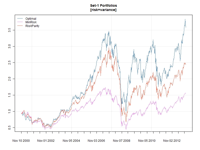
Finally, Figure 3 provides the ‘eye-catching’ illustration of terminal wealth trajectories of the various allocation models under the variance risk measure.
Set 2: Higher Diversity Universe
This is a more typical dataset for active asset allocation based on a more diverse universe of asset classes, though we are still limited in this application by readily available instruments and history within an open-data paradigm. The set covers the period June-2006 to December-2013, and I have again used weekly (Friday) returns. The backtest follows the exact methodology of Set 1.
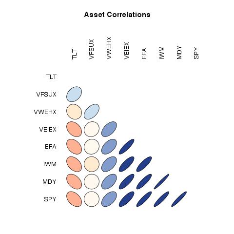
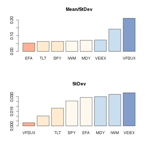
Figure 4 displays good diversification potential in terms of correlations, whilst Figure 5 provides an indication of the risk and risk-return profile of the dataset, with the same caveats as mentioned for Figure 2.
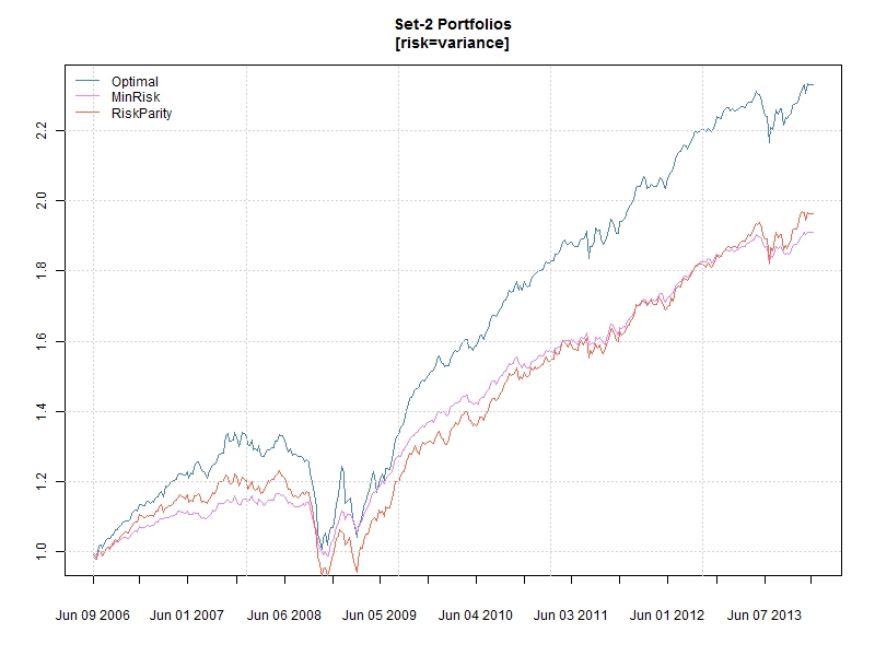
The results in Table 2 provide for some very interesting insights. The higher diversification potential of this dataset has resulted in an exact opposite ranking for the MR portfolio which now has the highest Sharpe ratio, though a much lower CAGR, and the OPT portfolio again beats the RP portfolio. However, the RP portfolio now comfortably outperforms the equal weight portfolio, in line with expectations, given that the risks in the unconditional dataset were not very close (unlike set 1).
Table-2
| SET-2 | RP[EV] | RP[MAD] | RP[LPM2] | RP[LPM4] | MR[EV] | MR[MAD] | MR[LPM2] | MR[LPM4] | OPT[EV] | OPT[MAD] | OPT[LPM2] | OPT[LPM4] | EW |
|---|---|---|---|---|---|---|---|---|---|---|---|---|---|
| CAGR | 9.35 | 9.38 | 9.29 | 9.37 | 8.95 | 8.98 | 8.91 | 8.96 | 11.87 | 11.55 | 11.47 | 12.25 | 10.41 |
| SD | 8.17 | 8.17 | 8.08 | 8.23 | 5.14 | 5.13 | 5.15 | 5.46 | 8.89 | 8.94 | 8.76 | 9.35 | 23.31 |
| Up | 60.46 | 60.20 | 60.46 | 59.95 | 62.24 | 61.48 | 62.24 | 64.29 | 65.31 | 65.56 | 65.56 | 66.58 | 54.08 |
| MaxDrawdown | 24.68 | 24.86 | 24.59 | 24.83 | 15.21 | 15.07 | 15.53 | 17.34 | 24.83 | 24.77 | 24.40 | 26.07 | 55.83 |
| CAPM[alpha] | 4.67 | 4.68 | 4.67 | 4.75 | 6.37 | 6.41 | 6.32 | 6.05 | 7.66 | 7.39 | 7.35 | 7.94 | |
| CAPM[beta] | 0.30 | 0.30 | 0.29 | 0.29 | 0.10 | 0.10 | 0.10 | 0.13 | 0.24 | 0.24 | 0.23 | 0.25 | |
| Timing | 0.73 | 0.73 | 0.73 | 0.73 | 0.34 | 0.34 | 0.35 | 0.45 | 0.64 | 0.63 | 0.63 | 0.63 | |
| Sharpe | 0.98 | 0.98 | 0.98 | 0.98 | 1.48 | 1.49 | 1.47 | 1.40 | 1.18 | 1.14 | 1.15 | 1.16 | 0.39 |
| Information | 0.99 | 1.00 | 0.99 | 0.99 | 1.49 | 1.50 | 1.48 | 1.41 | 1.20 | 1.15 | 1.17 | 1.18 | 0.39 |
| Calmar | 0.38 | 0.38 | 0.38 | 0.38 | 0.59 | 0.60 | 0.57 | 0.52 | 0.48 | 0.47 | 0.47 | 0.47 | 0.19 |
| Skew | -0.67 | -0.70 | -0.69 | -0.66 | -0.38 | -0.35 | -0.38 | -0.80 | -1.17 | -1.35 | -1.28 | -0.85 | -0.09 |
| Kurtosis | 3.16 | 3.16 | 3.33 | 3.54 | 4.75 | 4.73 | 4.74 | 5.71 | 7.39 | 7.88 | 8.13 | 9.02 | 6.48 |
Conclusions
It is certainly fashionable to publish about uncertainty of inputs in the portfolio literature. Michaud (1989) did it, DeMiguel, Garlappi and Uppal (2009) did it (see this blog for a critique), and so have the proponents of Risk Parity. I don’t see how an investment manager can justify the use of any of these methodologies since he is rewarded for the quality of his inputs (active bets), though they can and certainly should serve a role in sensitivity analysis. If everyone could just allocate resources without a forecast then we would not need investment/resource managers. Even with simple econometric based forecasts such as those generated from a ‘simple’ AR(1) model we still managed to beat the RP and EW portfolios. Perhaps a little more attention should be given to the modelling of the underlying dynamics and a little less to ‘fashionable’ trends in asset allocation and catchy phrases meant to provide yet another sales drive, particularly given the resulting highly levered bets on a certain asset class whose rally depends heavily on a printing press which is fast running out of steam.
Code
If you want the code to replicate the results or the RP code for use with parma, contact me by email stating your real name and affiliation.
References
Charnes, A., & Cooper, W. W. (1962). Programming with linear fractional functionals. Naval Research logistics quarterly, 9(3-4), 181-186.
Chaves, D., Hsu, J., Li, F., & Shakernia, O. (2012). Efficient Algorithms for Computing Risk Parity Portfolio Weights. The Journal of Investing, 21(3), 150-163.
DeMiguel, V., Garlappi, L., & Uppal, R. (2009). Optimal versus naive diversification: How inefficient is the 1/N portfolio strategy?. Review of Financial Studies, 22(5), 1915-1953.
Genest, C., Ghoudi, K., & Rivest, L. P. (1995). A semiparametric estimation procedure of dependence parameters in multivariate families of distributions. Biometrika, 82(3), 543-552.
Maillard, S., Roncalli, T., & Teïletche, J. (2010). The Properties of Equally Weighted Risk Contribution Portfolios. The Journal of Portfolio Management, 36(4), 60-70.
Michaud, R. O. (1989). The Markowitz optimization enigma: is’ optimized’optimal?. Financial Analysts Journal, 31-42.
Stoyanov, S. V., Rachev, S. T., & Fabozzi, F. J. (2007). Optimal financial portfolios. Applied Mathematical Finance, 14(5), 401-436.
Footnotes
\( ^{1} \) Risk, despite the numerous papers written on risk parity including the seminal one by Maillard, Roncalli and Teïletche (2010) (although the concept appears to have originated as far back as 1996 with Ray Dalio of Bridgewater Associates, with the actual term ‘Risk Parity’ coined by E.Qian of PanAgora in 2006) is certainly not equivalent to variance. It can be any number of measures deemed appropriate (see the parma vignette section for a discussion of risk and deviation measures), and this blog article shows how the parma package can be used to calculate RP under a number of different measures in addition to variance, including Mean Absolute Deviation (MAD) and Lower Partial Moments (LPM).
\( ^{2} \) The threshold was based on the portfolio mean which is a case with especially desirable properties as discussed in the parma vignette.
