This demonstration provides for an introduction to, and exposition of, some of the features of the rugarch package. See this post for latest developments.
require(rugarch)
data(sp500ret)
# create a cluster object to be used as part of this demonstration
cluster = makePSOCKcluster(15)
The GARCH model specification: ugarchspec
The ugarchspec function is the entry point for most of the modelling done in the rugarch package. This is where the model for the conditional mean, variance and distribution is defined, in addition to allowing the user to pass any starting or fixed parameters, the naming of which is described in the documentation.
spec = ugarchspec()
show(spec)
##
## *---------------------------------*
## *       GARCH Model Spec          *
## *---------------------------------*
##
## Conditional Variance Dynamics
## ------------------------------------
## GARCH Model          : sGARCH(1,1)
## Variance Targeting   : FALSE
##
## Conditional Mean Dynamics
## ------------------------------------
## Mean Model       : ARFIMA(1,0,1)
## Include Mean     : TRUE
## GARCH-in-Mean    : FALSE
##
## Conditional Distribution
## ------------------------------------
## Distribution     :  norm
## Includes Skew    :  FALSE
## Includes Shape   :  FALSE
## Includes Lambda  :  FALSE
This defines a basic ARMA(1,1)-GARCH(1,1) model, though there are many more options to choose from ranging from the type of GARCH model, the ARFIMAX-arch-in-mean specification and conditional distribution. In fact, and considering only the (1,1) order for the GARCH and ARMA models, there are 13440 possible combinations of models and model options to choose from:
nrow(expand.grid(GARCH = 1:14, VEX = 0:1, VT = 0:1, Mean = 0:1, ARCHM = 0:2, ARFIMA = 0:1, MEX = 0:1, DISTR = 1:10))
The returned object, of class uGARCHspec can take a set of starting or fixed parameters either at the initialization stage or afterwards by use of the setstart< – and setfixed< – methods. Let’s change the model to an eGARCH model with student distribution and set the student shape starting parameter to 5. Note that there is also a setbounds< – method for defining custom lower and upper bound for most of the parameters, and I’ll simply illustrate by changing the bounds for the student shape parameters from the default of (2.1, 100) to (4.1,30).
spec = ugarchspec(variance.model = list(model = 'eGARCH', garchOrder = c(2, 1)), distribution = 'std')
setstart(spec) < - list(shape = 5)
setbounds(spec)
If only a single value is passed to the bounds then this is treated as the lower bound setting. Once a specification is defined, there are a number of options available. If you want to estimate the parameters of the model, the ugarchfit method may be used, otherwise a specification with a complete model set of fixed parameters may be passed to other methods which will be described later.
Estimating a GARCH model: ugarchfit
The estimation of the model takes as argument the previously defined specification, a dataset conforming to a number of different formats described in the documentation, and some additional arguments relating to the type of solver used, its control parameters and an additional list of options (fit.control) which may be used to fine tune the estimation process in case of difficulty converging.
fit = ugarchfit(spec, sp500ret[1:1000, , drop = FALSE], solver = 'hybrid')
The types of solvers available are detailed in the documentation, where the choice of “hybrid” is in effect a safety strategy which starts with the default solver solnp, and then cycles through the other available solvers in case of non-convergence. This will likely catch 90% of estimation problems without having to adjust any of the solver.control or fit.control parameters, though this will vary depending on the type and length of your dataset and the choice of model (e.g. the “ALLGARCH” submodel of “fGARCH” is known to be notoriously difficult to estimate out of the box). The returned object of class uGARCHfit has a number of methods for manipulating it or passing it to other functions for further analysis. Basic methods are described in the table below:
| Method | Description | Options |
|---|---|---|
| coef | parameter estimates | |
| vcov | covariance matrix of the parameters | robust (logical) |
| infocriteria | information criteria | |
| nyblom | Hansen-Nyblom (1990) stability test (single and joint) | |
| gof | Vlaar and Palm (1993) adjusted goodness | groups (vector) |
| newsimpact | news impact curve x-y values for plotting | |
| signbias | Engle and Ng (1993) sign bias test | |
| likelihood | log-likelihood at estimated optimum | |
| sigma | conditional sigma | |
| fitted | conditional mean | |
| residuals | residuals | standardize (logical) |
| getspec | extract specification object used | |
| persistence | conditional variance persistence | |
| uncvariance | long run unconditional model variance | |
| uncmean | long run unconditional model mean | |
| halflife | conditional variance half life (same time scale as data) | |
| convergence | solver convergence flag | |
| plot | model plots (choice of 12) | which (1:12, ask, all) |
| show | results summary | |
| quantile | conditional quantile | probs |
| pit | conditional probability integral transformation |
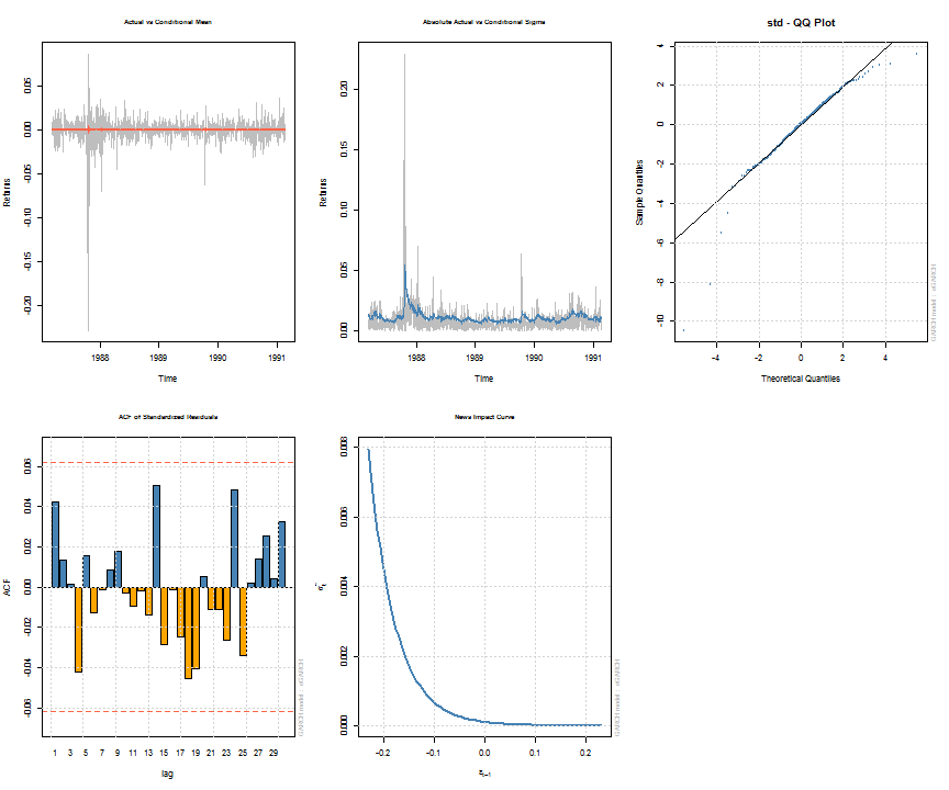
Note that some of the methods, such as uncvariance, uncmean, halflife and persistence can also be calculated by passing a suitably named vector of parameters with model/distribution details. This is explained more fully in the documentation, whilst the formulae and calculations are found in the package’s vignette. The following shows a summary of the estimated object and a few plots for illustration. The diagnostic tests printed with the summary are described in detail in the vignette.
##
## *---------------------------------*
## *          GARCH Model Fit        *
## *---------------------------------*
##
## Conditional Variance Dynamics
## -----------------------------------
## GARCH Model  : eGARCH(2,1)
## Mean Model   : ARFIMA(1,0,1)
## Distribution : std
##
## Optimal Parameters
## ------------------------------------
##         Estimate  Std. Error  t value Pr(>|t|)
## mu      0.000668    0.000274   2.4397 0.014698
## ar1    -0.677808    0.261666  -2.5904 0.009588
## ma1     0.701097    0.253432   2.7664 0.005668
## omega  -0.271972    0.112887  -2.4092 0.015986
## alpha1 -0.198962    0.059386  -3.3503 0.000807
## alpha2  0.130487    0.059794   2.1823 0.029089
## beta1   0.970496    0.012318  78.7851 0.000000
## gamma1 -0.009355    0.077629  -0.1205 0.904085
## gamma2  0.125453    0.080531   1.5578 0.119273
## shape   4.649923    0.686848   6.7699 0.000000
##
## Robust Standard Errors:
##         Estimate  Std. Error  t value Pr(>|t|)
## mu      0.000668    0.000266  2.50648 0.012194
## ar1    -0.677808    0.143561 -4.72140 0.000002
## ma1     0.701097    0.139159  5.03809 0.000000
## omega  -0.271972    0.150634 -1.80551 0.070995
## alpha1 -0.198962    0.059808 -3.32669 0.000879
## alpha2  0.130487    0.056811  2.29685 0.021627
## beta1   0.970496    0.016573 58.55853 0.000000
## gamma1 -0.009355    0.070989 -0.13177 0.895163
## gamma2  0.125453    0.075238  1.66741 0.095433
## shape   4.649923    0.857054  5.42547 0.000000
##
## LogLikelihood : 3205
##
## Information Criteria
## ------------------------------------
##
## Akaike       -6.3903
## Bayes        -6.3412
## Shibata      -6.3905
## Hannan-Quinn -6.3716
##
## Q-Statistics on Standardized Residuals
## ------------------------------------
##               statistic p-value
## Lag[1]            1.809  0.1786
## Lag[p+q+1][3]     2.005  0.1568
## Lag[p+q+5][7]     4.285  0.5092
## d.o.f=2
## H0 : No serial correlation
##
## Q-Statistics on Standardized Squared Residuals
## ------------------------------------
##               statistic p-value
## Lag[1]            2.675 0.10192
## Lag[p+q+1][4]     3.915 0.04787
## Lag[p+q+5][8]     4.220 0.51819
## d.o.f=3
##
## ARCH LM Tests
## ------------------------------------
##              Statistic DoF P-Value
## ARCH Lag[2]      2.749   2  0.2530
## ARCH Lag[5]      3.805   5  0.5778
## ARCH Lag[10]     5.377  10  0.8646
##
## Nyblom stability test
## ------------------------------------
## Joint Statistic:  1.433
## Individual Statistics:
## mu     0.07859
## ar1    0.06532
## ma1    0.06596
## omega  0.19861
## alpha1 0.31446
## alpha2 0.34612
## beta1  0.19466
## gamma1 0.13448
## gamma2 0.19960
## shape  0.24821
##
## Asymptotic Critical Values (10% 5% 1%)
## Joint Statistic:          2.29 2.54 3.05
## Individual Statistic:     0.35 0.47 0.75
##
## Sign Bias Test
## ------------------------------------
##                    t-value      prob sig
## Sign Bias           0.3613 0.7179747
## Negative Sign Bias  3.4390 0.0006082 ***
## Positive Sign Bias  0.1949 0.8455070
## Joint Effect       12.8658 0.0049359 ***
##
##
## Adjusted Pearson Goodness-of-Fit Test:
## ------------------------------------
##   group statistic p-value(g-1)
## 1    20     28.88       0.0679
## 2    30     33.62       0.2534
## 3    40     49.60       0.1190
## 4    50     61.90       0.1021
##
##
## Elapsed time : 0.7354
Filtering new data: ugarchfilter
There are situations where new data has arrived (or is streaming in), or the coefficients for a model already exist, and you wish to extract new values from the model. The ugarchfilter method takes a uGARCHspec object which has an appropriately set fixed list of named parameters for that model, and filters the new data with these parameters. Continuing from the previous example of having estimated a model, the example below shows how a specification object can be retrieved from a uGARCHfit object and the estimated parameters fixed to it:
spec = getspec(fit)
setfixed(spec) < - as.list(coef(fit))
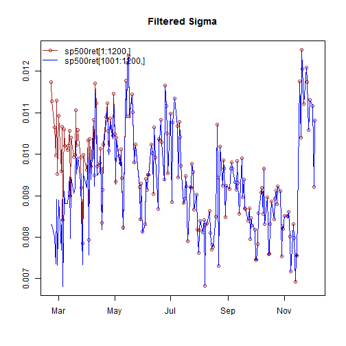
The option of filtering new data with this specification creates a small challenge since GARCH models need to be initialized to start the recursion. One way to achieve continuity between the previous values of the dataset is to append the new values to the old dataset and indicate to the method the size of the original data (otherwise the mean of the squared residuals of the passed dataset is used). The following example clarifies:
filt1 = ugarchfilter(spec, sp500ret[1:1200, ], n.old = 1000)
filt2 = ugarchfilter(spec, sp500ret[1001:1200, ])
As can be seen from the plot, it takes a few periods before the new data, without the old data appended, to converge, as a result of the initialization problem. A future update may allow the setting of a user value for the initialization in order to avoid the use of appending new to old. The resulting object, of class uGARCHfilter has the same methods available as that for the uGARCHfit class, details of which were given in the table above.
Parameter uncertainty and simulated density: ugarchdistribution
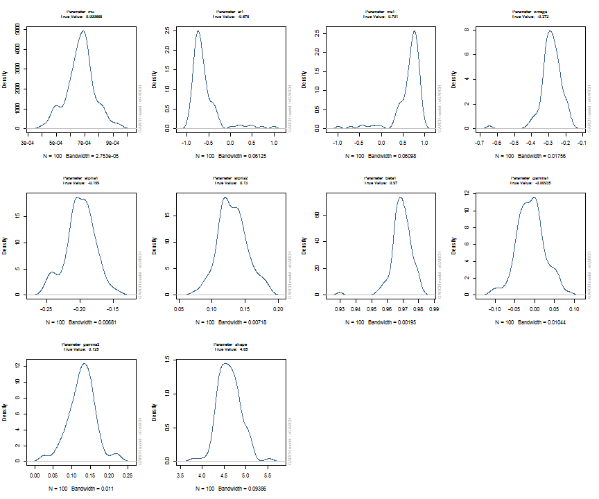
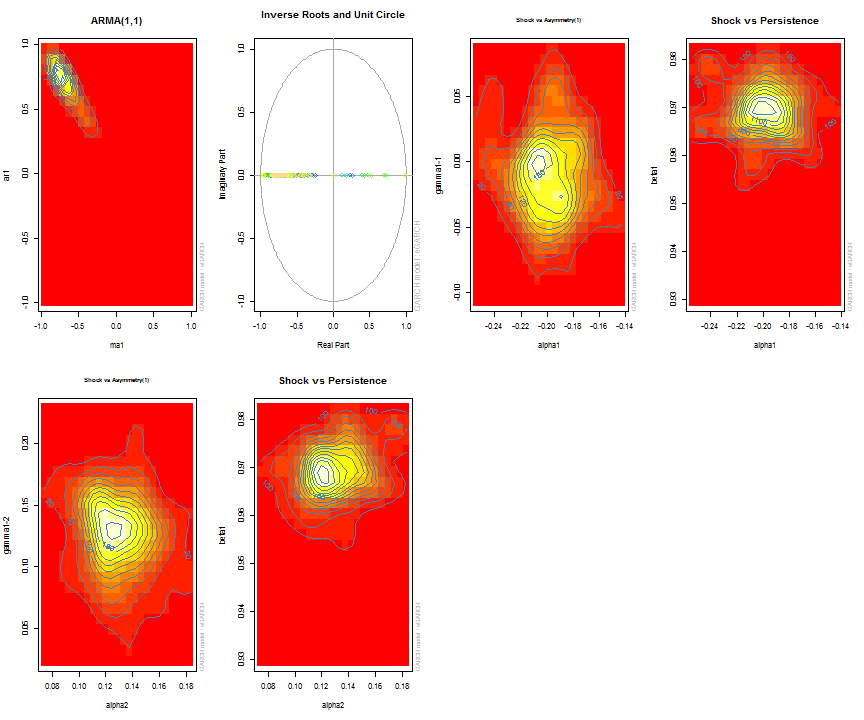
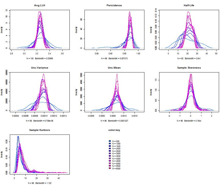
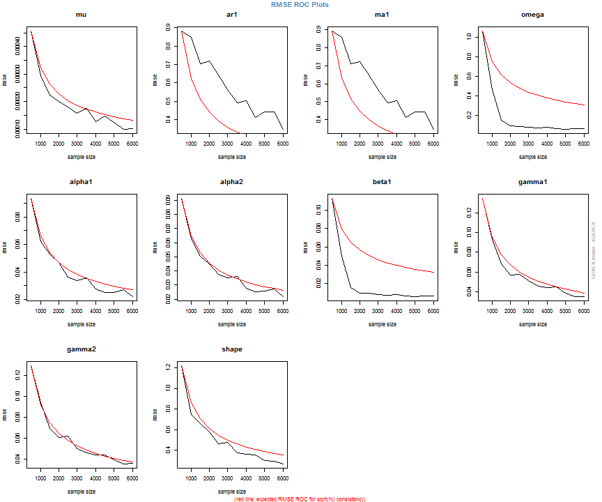
The issue of parameter uncertainty is one often neglected in practice. The ugarchdistribution method enables the generation of the simulated parameter density of a set of parameters from a model, the Root Mean Squared Error (RMSE) of true versus estimated parameters in relation to the data size, and various other interesting views on the direct interaction between model parameters and indirect influence on such values as persistence, half-life etc. The method takes either an object of class uGARCHfit or one of class uGARCHspec with fixed parameters. The following example illustrates with a number of plots which are available once the resulting object of class uGARCHdistribution is obtained, with optional argument the window number for which to return results for.
gd = ugarchdistribution(fit, n.sim = 500, recursive = TRUE, recursive.length = 6000, recursive.window = 500, m.sim = 100, solver = 'hybrid', cluster = cluster)
show(gd)
plot(gd, which = 1, window = 12)
plot(gd, which = 2, window = 12)
plot(gd, which = 3, window = 12)
plot(gd, which = 4, window = 12)
##
## *------------------------------------*
## *    GARCH Parameter Distribution    *
## *------------------------------------*
## Model : eGARCH
## No. Paths (m.sim) : 100
## Length of Paths (n.sim) : 500
## Recursive : TRUE
## Recursive Length : 6000
## Recursive Window : 500
##
## Coefficients: True vs Simulation Mean (Window-n)
##                     mu       ar1      ma1    omega   alpha1  alpha2   beta1     gamma1  gamma2  shape
## true-coef   0.00066774 -0.677808 0.701097 -0.27197 -0.19896 0.13049 0.97050 -0.0093545 0.12545 4.6499
## window-500  0.00064907 -0.050559 0.072872 -0.52134 -0.19418 0.11457 0.94390 -0.0584706 0.15195 4.8854
## window-1000 0.00063383 -0.139771 0.163514 -0.39555 -0.19664 0.12056 0.95702 -0.0153573 0.12632 4.8159
## window-1500 0.00066351 -0.270665 0.292857 -0.32520 -0.20155 0.12772 0.96473 -0.0231710 0.13741 4.7509
## window-2000 0.00064268 -0.286364 0.311060 -0.29546 -0.20100 0.13123 0.96795 -0.0217545 0.13303 4.7465
## window-2500 0.00065872 -0.307483 0.332827 -0.27606 -0.19668 0.12840 0.97008 -0.0148314 0.12540 4.7435
## window-3000 0.00066431 -0.388779 0.412578 -0.28369 -0.19634 0.12778 0.96928 -0.0162039 0.12664 4.8123
## window-3500 0.00067496 -0.470185 0.495252 -0.28922 -0.20132 0.13154 0.96860 -0.0138806 0.13106 4.6607
## window-4000 0.00066358 -0.461820 0.486043 -0.29191 -0.19761 0.12802 0.96837 -0.0142306 0.13258 4.7495
## window-4500 0.00065904 -0.522260 0.547011 -0.27890 -0.19554 0.12565 0.96980 -0.0167349 0.12871 4.7248
## window-5000 0.00066542 -0.500693 0.525181 -0.27855 -0.19722 0.12740 0.96979 -0.0116117 0.12605 4.6822
## window-5500 0.00067243 -0.505235 0.529267 -0.28570 -0.19974 0.12949 0.96899 -0.0088217 0.12397 4.6911
## window-6000 0.00067057 -0.595439 0.618946 -0.28508 -0.19974 0.13092 0.96904 -0.0096572 0.12670 4.6209
Long range and rolling forecasts: ugarchforecast
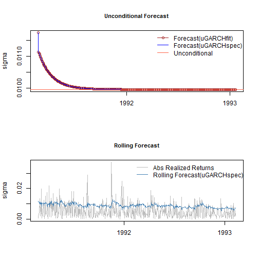
Forecasting in rugarch, allows for both n.ahead unconditional forecasts as well as rolling forecasts based on the use of the out.sample option. It has two dispatch methods allowing the user to call it with either an object of class uGARCHfit (in which case the data argument is ignored), or a specification object of class uGARCHspec (in which case the data is required) with fixed parameters. In the latter case, the data is first passed through the ugarchfilter function prior to initializing the forecast. Forecast in GARCH models is critically dependent on the expected value of the innovations and hence the density chosen. One step ahead forecasts are based on the value of the previous data, while n-step ahead (n>1) are based on the unconditional expectation of the models. The ability to roll the forecast 1 step at a time is implemented with the n.roll argument which controls how many times to roll the n.ahead forecast. The default argument of n.roll = 0 denotes no rolling and returns the standard n.ahead forecast. Critically, since n.roll depends on data being available from which to base the rolling forecast, the ugarchfit method needs to be called with the argument out.sample being at least as large as the n.roll argument, or in the case of a specification being used instead, the out.sample argument directly in the forecast function for use with the data. The following example illustrates:
forc1 = ugarchforecast(fit, n.ahead = 500)
forc2 = ugarchforecast(spec, n.ahead = 500, data = sp500ret[1:1000, , drop = FALSE])
forc3 = ugarchforecast(spec, n.ahead = 1, n.roll = 499, data = sp500ret[1:1500, , drop = FALSE], out.sample = 500)
f1 = as.data.frame(forc1)
f2 = as.data.frame(forc2)
f3 = t(as.data.frame(forc3, which = 'sigma', rollframe = 'all', aligned = FALSE))
U = uncvariance(fit)^0.5
There are a number of methods for extracting the forecasts, with each one allowing for additional options in order to handle complex setups such as n.ahead>1 combined with the n.roll>0. These are thoroughly described in the documentation together with some optional plot and summary methods. Finally note that since the n.roll option starts at zero (i.e. no roll), and given a default forecast of n.ahead=1, a rolling 1-ahead forecast of 500 points as above would require setting n.roll = 499 (i.e. 0:499). The next section describes a variation of the rolling forecast whereby it is possible to re-estimate the model every n periods.
Backtesting using rolling estimation and forecasts: ugarchroll
In backtesting risk models, it is important to re-estimate a model every so many periods, in order to capture any time variation/change in the parameters as a result of any number of factors which I will not go into here. Of particular importance, when using skewed and shaped distributions, is the variation in these parameter as a result of time variation in higher moments not captured by conventional GARCH models. The ugarchroll method allows for the generation of 1-ahead rolling forecasts and periodic re-estimation of the model, given either a moving data window (where the window size can be chosen), or an expanding window. The resulting object contains the forecast conditional density, namely the conditional mean, sigma, skew, shape and the realized data for the period under consideration from which any number of tests can be performed. Crucially, it takes advantage of parallel estimation given a user supplied cluster object created from the parallel package. The following example provides for an illustration of the method and its potential.
spec = ugarchspec(variance.model = list(model = 'gjrGARCH', garchOrder = c(2, 1)), distribution = 'jsu')
roll = ugarchroll(spec, sp500ret, forecast.length = 1000, refit.every = 50, refit.window = 'moving', window.size = 1200, calculate.VaR = FALSE, keep.coef = TRUE, cluster = cluster)
A key feature of this method is the existence of a rescue method called resume which allows the resumption of the estimation when there are non-converged windows, by submitting the resulting object into resume with the option of using a different solver, control parameters etc. This process can be continued until all windows converge, thus not wasting time and resources by having to resubmit the whole problem from scratch.
show(roll)
##
## *-------------------------------------*
## *              GARCH Roll             *
## *-------------------------------------*
## No.Refits        : 20
## Refit Horizon    : 50
## No.Forecasts : 1000
## GARCH Model      : gjrGARCH(2,1)
## Distribution : jsu
##
## Forecast Density:
##                Mu  Sigma   Skew Shape Shape(GIG) Realized
## 2005-02-10  1e-04 0.0067 -1.435 8.161          0   0.0042
## 2005-02-11 -2e-04 0.0067 -1.435 8.161          0   0.0069
## 2005-02-14 -6e-04 0.0066 -1.435 8.161          0   0.0007
## 2005-02-15 -5e-04 0.0064 -1.435 8.161          0   0.0033
## 2005-02-16 -5e-04 0.0063 -1.435 8.161          0   0.0002
## 2005-02-17 -4e-04 0.0062 -1.435 8.161          0  -0.0080
##
## ..........................
##                 Mu  Sigma    Skew Shape Shape(GIG) Realized
## 2009-01-23  0.0020 0.0293 -0.7756 2.275          0   0.0054
## 2009-01-26  0.0008 0.0287 -0.7756 2.275          0   0.0055
## 2009-01-27 -0.0001 0.0274 -0.7756 2.275          0   0.0109
## 2009-01-28 -0.0013 0.0262 -0.7756 2.275          0   0.0330
## 2009-01-29 -0.0047 0.0250 -0.7756 2.275          0  -0.0337
## 2009-01-30  0.0010 0.0235 -0.7756 2.275          0  -0.0231
##
## Elapsed: 8.898 secs
head(fd < - as.data.frame(roll, which = 'density'))
##                    Mu    Sigma   Skew Shape Shape(GIG)   Realized
## 2005-02-10  7.266e-05 0.006671 -1.435 8.161          0  0.0042026
## 2005-02-11 -2.447e-04 0.006711 -1.435 8.161          0  0.0069017
## 2005-02-14 -5.597e-04 0.006567 -1.435 8.161          0  0.0006967
## 2005-02-15 -4.515e-04 0.006432 -1.435 8.161          0  0.0032944
## 2005-02-16 -5.107e-04 0.006304 -1.435 8.161          0  0.0001818
## 2005-02-17 -3.982e-04 0.006183 -1.435 8.161          0 -0.0079550
The rugarch package contains a set of functions to work with the standardized conditional distributions implemented. These are pdist (distribution), ddist (density), qdist (quantile) and rdist (random number generation), in addition to dskewness and dkurtosis to return the conditional density skewness and kurtosis values. Given the returned density forecast data.frame (fd), it is pretty simple to calculate any measure on the density. The following example calculates the VaR and Expected Shortfall which are then passed to two tests typically used to evaluate risk models.
VAR1 = fd[, 'Mu'] + qdist('jsu', 0.01, 0, 1, skew = fd[, 'Skew'], shape = fd[, 'Shape']) * fd[, 'Sigma']
VAR5 = fd[, 'Mu'] + qdist('jsu', 0.05, 0, 1, skew = fd[, 'Skew'], shape = fd[, 'Shape']) * fd[, 'Sigma']
PIT = pdist('jsu', (fd[, 'Realized'] - fd[, 'Mu'])/fd[, 'Sigma'], mu = 0, sigma = 1, fd[, 'Skew'], shape = fd[, 'Shape'])
VT1 = VaRTest(0.01, VaR = VAR1, actual = fd[, 'Realized'])
VT5 = VaRTest(0.05, VaR = VAR5, actual = fd[, 'Realized'])
# calculate ES
f = function(x, skew, shape) qdist('jsu', p = x, mu = 0, sigma = 1, skew = skew, shape = shape)
ES5 = apply(fd, 1, function(x) x['Mu'] + x['Sigma'] * integrate(f, 0, 0.05, skew = x['Skew'], shape = x['Shape'])$value)
ES1 = apply(fd, 1, function(x) x['Mu'] + x['Sigma'] * integrate(f, 0, 0.01, skew = x['Skew'], shape = x['Shape'])$value)
ET5 = ESTest(alpha = 0.05, actual = fd[, 'Realized'], ES = ES5, VaR = VAR5, conf.level = 0.95)
ET1 = ESTest(alpha = 0.01, actual = fd[, 'Realized'], ES = ES1, VaR = VAR1, conf.level = 0.95)
##
##                             VaR_1             VaR_5
## expected.exceed                10                50
## actual.exceed                  17                61
## cc.LRstat                  4.6796             3.456
## cc.critical                5.9915            5.9915
## cc.LRp                     0.0963            0.1776
## cc.Decision     Fail to Reject H0 Fail to Reject H0
##
##                              ES_1              ES_5
## p.value                         0                 0
## Decision                Reject H0         Reject H0
## $H1: 'Mean of Excess Violations of VaR is greater than zero'
Forecasting with the GARCH bootstrap: ugarchboot
There are two main sources of uncertainty about n.ahead forecasting from GARCH models, namely that arising from the form of the predictive density and due to parameter estimation. The bootstrap method considered in the ugarchboot method, is based on resampling innovations from either the empirical, semi-parametric (spd package) or kernel fitted distribution (ks package) of the estimated GARCH model to generate future realizations of the series and sigma. The “full” method, based on the referenced paper by Pascual, Romo and Ruiz (2006), takes into account parameter uncertainty by building a simulated distribution of the parameters through simulation and re-estimation. This process, while more accurate, is very time consuming. The “partial” method, only considers distribution uncertainty and while faster, will not generate prediction intervals for the sigma 1-ahead forecast for which only the parameter uncertainty is relevant in GARCH type models. As in the case of the ugarchforecast method, either an object of class uGARCHfit or one of uGARCHspec with fixed parameters is accepted.
Simulating GARCH models: ugarchsim and ugarchpath
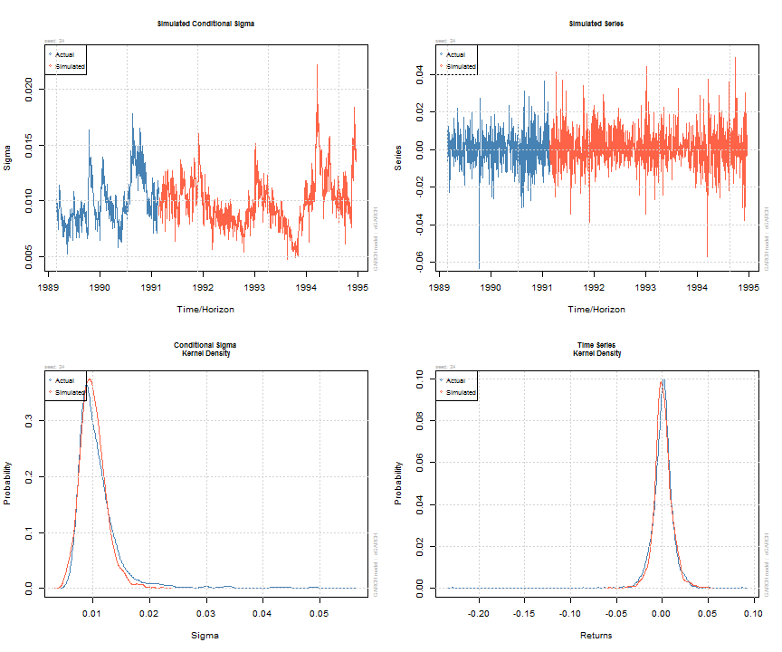
Simulation of GARCH models may be carried out either directly on an object of class uGARCHfit (in which case use the ugarchsim method) else on an object of class uGARCHspec with fixed parameters (in which case use the ugarchpath method). There is an option to set the simulation recursion starting method to either the model’s unconditional values (e.g. see uncvariance and uncmean), or the data sample’s last values. Simulation can return an n.sim (horizon) by m.sim (number of separate simulations of size n.sim) based result, use a custom defined random number sampler or set of pre-recorded innovations (custom.dist option), and make use of pre-sampled external regressor data for use with models which were defined with such (mexsimdata for conditional mean and vexsimdata for conditional variance). Replication of results is achieved by passing an appropriate integer to rseed in the function’s arguments. As with most functionality in rugarch, most of the work is done in either C or Rcpp for speed.
sim = ugarchsim(fit, n.sim = 1000, m.sim = 25, rseed = 1:25)
simSig = as.data.frame(sim, which = 'sigma')
simSer = as.data.frame(sim, which = 'series')
show(sim)
##
## *------------------------------------*
## *       GARCH Model Simulation       *
## *------------------------------------*
## Model : eGARCH
## Horizon:  1000
## Simulations: 25
##               Seed Sigma2.Mean Sigma2.Min Sigma2.Max Series.Mean Series.Min Series.Max
## sim1             1    1.11e-04   2.20e-05   0.000491    0.000838    -0.0607     0.0629
## sim2             2    1.06e-04   2.79e-05   0.000360    0.000764    -0.0533     0.0702
## sim3             3    1.06e-04   2.56e-05   0.000373    0.000672    -0.0412     0.0457
## sim4             4    9.33e-05   2.36e-05   0.000246    0.000855    -0.0499     0.0612
## sim5             5    1.11e-04   2.83e-05   0.000366    0.000658    -0.0588     0.0764
## sim6             6    1.02e-04   2.49e-05   0.000361    0.001096    -0.0554     0.0486
## sim7             7    1.39e-04   2.24e-05   0.000451    0.000246    -0.0694     0.0819
## sim8             8    1.20e-04   2.69e-05   0.000374    0.000815    -0.0621     0.0722
## sim9             9    9.83e-05   2.86e-05   0.000270    0.000761    -0.0510     0.0434
## sim10           10    1.31e-04   3.17e-05   0.000602    0.000416    -0.0556     0.0613
## sim11           11    1.01e-04   1.87e-05   0.000253    0.000912    -0.0357     0.0766
## sim12           12    1.04e-04   2.53e-05   0.000403    0.000890    -0.0401     0.0790
## sim13           13    9.77e-05   1.47e-05   0.000378    0.001107    -0.0433     0.0542
## sim14           14    1.48e-04   3.65e-05   0.000476    0.000232    -0.0552     0.0806
## sim15           15    1.12e-04   2.62e-05   0.000432    0.000621    -0.0517     0.0625
## sim16           16    1.18e-04   2.51e-05   0.000624    0.000812    -0.0817     0.0508
## sim17           17    8.68e-05   1.87e-05   0.000235    0.001491    -0.0489     0.0444
## sim18           18    1.47e-04   3.72e-05   0.000673    0.000306    -0.0594     0.0774
## sim19           19    1.08e-04   2.65e-05   0.000319    0.000392    -0.0579     0.0931
## sim20           20    1.14e-04   3.08e-05   0.000537    0.000640    -0.0625     0.0489
## sim21           21    9.11e-05   1.34e-05   0.000341    0.000872    -0.0468     0.0551
## sim22           22    7.99e-05   2.25e-05   0.000192    0.001239    -0.0427     0.0702
## sim23           23    1.22e-04   2.52e-05   0.000427    0.000449    -0.0606     0.0652
## sim24           24    1.05e-04   2.21e-05   0.000492    0.000904    -0.0572     0.0492
## sim25           25    1.00e-04   3.40e-05   0.000380    0.000222    -0.0652     0.0401
## Mean(All)        0    1.10e-04   2.55e-05   0.000402    0.000728    -0.0547     0.0628
## Actual           0    1.43e-04   2.73e-05   0.002989    0.000236    -0.2290     0.0871
## Unconditional    0    9.92e-05         NA         NA    0.000668         NA         NA
##
plot(sim, which = 'all', m.sim = 24)
Diagnostic, misspecification and operational tests…and some benchmarks
The rugarch package includes a number of diagnostic, misspecification and operational risk and forecast evaluation tests. The diagnostic tests were already shown in the output to the estimated model in the section on ugarchfit. The misspecification tests currently included in the package are the GMM (Orthogonal Moments) test of Hansen (1982) and non parametric Portmanteau type test of Hong and Li (2005), both of which are described in detail in the package’s vignette. More operational type tests include the density forecast test and tail test of Berkowitz (2001), VaR exceedances test of Christoffersen (1998), VaR Duration of Christoffersen and Pelletier (2004), Expected Shortfall of McNeil et al.(2000), and the Directional Accuracy (DAC) tests of Pesaran and Timmermann (1992), and Anatolyev and Gerko (2005). There is also some unexported functionality in the package for working with the VaR loss function described in González-Rivera et al.(2004) and the MCS test of Hansen, Lunde and Nasson (2011) which the advanced reader can investigate by looking at the source. Finally, there is a small GARCH benchmark function which compares some of the models estimated in rugarch with either a commercial implementation, or the published analytic results of Bollerslev and Ghysels(1996) for the standard and exponential GARCH models on the DM/BP (dmbp) data. The Log Relative Error test which is output indicates the number of significant digits (in the coefficients and standard errors) of agreement between the benchmark and the rugarch package estimate:
print(ugarchbench('published'))
##
## Bollerslev-Ghysels Benchmark 1/2: mu-ARMA(0,0)-sGARCH(1,1)-norm
##
## parameters:
##                  mu   omega alpha1  beta1
## rugarch   -0.006227 0.01076 0.1534 0.8059
## benchmark -0.006190 0.01076 0.1531 0.8060
##
## standard errors:
##                 mu    omega  alpha1   beta1
## rugarch   0.008467 0.002853 0.02658 0.03357
## benchmark 0.008462 0.002853 0.02652 0.03355
##
## Log Relative Error Test:
##        coef st.error
## mu    2.223    3.251
## omega 3.817    4.281
## alpha 2.761    2.663
## beta  3.975    3.411
##
## Bollerslev-Ghysels Benchmark 2/2: mu-ARMA(0,0)-eGARCH(1,1)-norm
##
## parameters:
##                 mu   omega   alpha1  beta1 gamma1
## rugarch   -0.01171 -0.1264 -0.03831 0.9126 0.3329
## benchmark -0.01168 -0.1263 -0.03846 0.9127 0.3331
##
## standard errors:
##                 mu   omega alpha1  beta1  gamma1
## rugarch   0.008326 0.02723 0.0183 0.0162 0.03876
## benchmark 0.008860 0.02850 0.0192 0.0168 0.04060
##
## Log Relative Error Test:
##        coef st.error
## mu    2.519    1.220
## omega 3.239    1.352
## alpha 2.407    1.331
## gamma 4.153    1.444
## beta  3.377    1.343
The standalone ARFIMAX model and methods
In addition to the ARFIMAX-GARCH models, the rugarch package includes a set of standalone ARFIMAX (constant variance) methods, including specification of the model, estimation, forecasting, simulation and rolling estimation/forecast. In this example, I will instead focus on the autoarfima function which has become quite popular in related packages. This allows for either a partial evaluation of consecutive orders of AR and MA, or a full evaluation of all possible combinations within the consecutive orders (thus enumerating the complete space of MA and AR orders). The use of parallel resources, via the passing of a cluster object is highly recommended.
AC = autoarfima(as.numeric(sp500ret[1:1000, 1]), ar.max = 5, ma.max = 5, criterion = 'HQIC', method = 'full', arfima = FALSE, include.mean = NULL, distribution.model = 'norm', cluster = cluster, solver = 'solnp')
show(head(AC$rank.matrix))
##
##   ar1 ar2 ar3 ar4 ar5 ma1 ma2 ma3 ma4 ma5 im arf   HQIC converged
## 1   1   1   0   0   1   0   1   0   0   1  1   0 -5.757         1
## 2   0   1   0   0   1   1   1   1   0   1  1   0 -5.755         1
## 3   0   0   0   1   0   0   1   0   0   1  0   0 -5.755         1
## 4   0   0   0   0   0   0   1   0   1   1  0   0 -5.755         1
## 5   0   1   0   1   0   0   0   0   0   1  0   0 -5.755         1
## 6   0   1   0   0   0   0   0   0   1   1  0   0 -5.755         1
The results indicate that an ARMA model with AR orders 1,2 and 5 and MA orders 2 and 5, including a mean intercept (im) is the best fitting model under the HQ information criterion. The best estimated model is also returned and is the slot named “fit” on the list. Note that in order to specify non-consecutive orders in either the GARCH or ARMA models, you need to set the order(s) you want to exclude to zero in the fixed parameters list of the specification. For example, an ARMA model as the one returned above would be specified as:
spec = arfimaspec(mean.model = list(armaOrder = c(5, 5)))
setfixed(spec) < - list(ar3 = 0, ar4 = 0, ma1 = 0, ma3 = 0, ma4 = 0)
Possible Future Developments
In order of interest:
- The jump GARCH model
- More tests
- Realized Vol (completed)
- A package GUI
References
Anatolyev, S., & Gerko, A. (2005). A trading approach to testing for predictability. Journal of Business & Economic Statistics, 23(4), 455-461.
Berkowitz, J. (2001). Testing density forecasts, with applications to risk management. Journal of Business & Economic Statistics, 19(4), 465-474.
Bollerslev, T., & Ghysels, E. (1996). Periodic autoregressive conditional heteroscedasticity. Journal of Business & Economic Statistics, 14(2), 139-151.
Christoffersen, P. F. (1998). Evaluating Interval Forecasts. International Economic Review, 39(4), 841-62.
Christoffersen, P., & Pelletier, D. (2004). Backtesting value-at-risk: A duration-based approach. Journal of Financial Econometrics, 2(1), 84-108.
González-Rivera, G., Lee, T. H., & Mishra, S. (2004). Forecasting volatility: A reality check based on option pricing, utility function, value-at-risk, and predictive likelihood. International Journal of Forecasting, 20(4), 629-645.
Hansen, L. P. (1982). Large sample properties of generalized method of moments estimators. Econometrica: Journal of the Econometric Society, 1029-1054.
Hansen, P. R., Lunde, A., & Nason, J. M. (2011). The model confidence set. Econometrica, 79(2), 453-497.
Hong, Y., & Li, H. (2005). Nonparametric specification testing for continuous-time models with applications to term structure of interest rates. Review of Financial Studies, 18(1), 37-84.
McNeil, A. J., & Frey, R. (2000). Estimation of tail-related risk measures for heteroscedastic financial time series: an extreme value approach. Journal of empirical finance, 7(3), 271-300.
Pesaran, M. H., & Timmermann, A. (1992). A simple nonparametric test of predictive performance. Journal of Business & Economic Statistics, 10(4), 461-465.
Pascual, L., Romo, J., & Ruiz, E. (2006). Bootstrap prediction for returns and volatilities in GARCH models. Computational Statistics & Data Analysis, 50(9), 2293-2312.
