Since the last release of rugarch on CRAN (ver 1.0-16), there have been many changes and new features in the development version of the package (ver 1.01-5). First, development of the package (and svn) has been moved to google code from r-forge. Second, the package now features exclusive use of xts based time series for input data and also outputs some of the results as xts as well. The sections that follow highlight some of the key changes to the package which I hope will make it easier to work with.
Extractor Methods
sigma, fitted and residuals
The main extractor method is no longer the as.data.frame, but instead, sigma and fitted will now extract the conditional sigma (GARCH) and mean (ARFIMA) values from all objects. The old extractor methods are now mostly deprecated, with the exception of certain classes where it still makes sense to use them (i.e. uGARCHroll, uGARCHdistribution, uGARCHboot).
library(rugarch)
data(sp500ret)
fit = ugarchfit(ugarchspec(), sp500ret, out.sample = 10)
c(is(sigma((fit))), is(fitted(fit)), is(residuals(fit)))
## [1] 'xts' 'xts' 'xts'
##
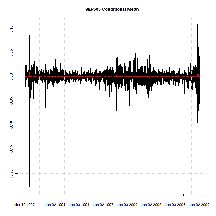
plot(xts(fit@model$modeldata$data, fit@model$modeldata$index), auto.grid = FALSE,
minor.ticks = FALSE, main = 'S&P500 Conditional Mean')
lines(fitted(fit), col = 2)
grid()
plot(xts(abs(fit@model$modeldata$data), fit@model$modeldata$index), auto.grid = FALSE,
minor.ticks = FALSE, main = 'S&P500 Conditional Sigma', col = 'grey')
lines(sigma(fit), col = 'steelblue')
grid()
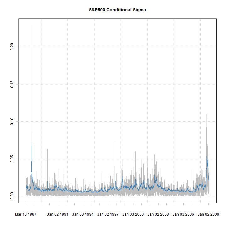
Apart from getting the nice xts charts, rugarch can now handle any type of time-formatted data (which can be coerced to xts) including intraday.
A key change has also been made to the output of the forecast class (uGARCHforecast) which merits particular attention. Because rugarch allows to combine both rolling and unconditional forecasts, this creates a rather challenging problem in how to meaningfully output the results, with simple extractor methods such as sigma and fitted. The output in this case will be an n.ahead by (n.roll+1) matrix, where the column headings are now the T+0 dates, since they will always exist to use within a forecast framework, whilst the row names are labelled as T+1, T+2, …,T+n.ahead. The following example illustrates, and shows some simple solutions to deal with portraying n.ahead dates which are completely in the future (i.e. not in the available out of sample testing period).
f = ugarchforecast(fit, n.ahead = 25, n.roll = 9)
sf = sigma(f)
head(sf)
##     2009-01-15 2009-01-16 2009-01-20 2009-01-21 2009-01-22 2009-01-23  2009-01-26 2009-01-27 2009-01-28 2009-01-29
## T+1    0.02176    0.02078    0.02587    0.02730    0.02646    0.02519     0.02400    0.02301    0.02388    0.02487
## T+2    0.02171    0.02073    0.02580    0.02722    0.02638    0.02512     0.02393    0.02295    0.02382    0.02480
## T+3    0.02166    0.02069    0.02573    0.02714    0.02630    0.02505     0.02387    0.02289    0.02375    0.02473
## T+4    0.02160    0.02064    0.02565    0.02706    0.02623    0.02498     0.02380    0.02283    0.02369    0.02466
## T+5    0.02155    0.02059    0.02558    0.02697    0.02615    0.02491     0.02374    0.02277    0.02363    0.02459
## T+6    0.02150    0.02054    0.02550    0.02689    0.02607    0.02484     0.02368    0.02271    0.02356    0.02452
Therefore, the column headings are the T+0 dates i.e. the date at which the forecast was made. There are 10 columns since the n.roll option is zero based. To create an xts representation of only the rolling output is very simple:
print(sf[1, ])
## 2009-01-15 2009-01-16 2009-01-20 2009-01-21 2009-01-22 2009-01-23 2009-01-26 2009-01-27 2009-01-28 2009-01-29
##    0.02176    0.02078    0.02587    0.02730    0.02646    0.02519    0.02400    0.02301    0.02388    0.02487
##
print(f.roll < - as.xts(sf[1, ]))
##               [,1]
## 2009-01-15 0.02176
## 2009-01-16 0.02078
## 2009-01-20 0.02587
## 2009-01-21 0.02730
## 2009-01-22 0.02646
## 2009-01-23 0.02519
## 2009-01-26 0.02400
## 2009-01-27 0.02301
## 2009-01-28 0.02388
## 2009-01-29 0.02487
This gives the T+0 dates. If you want to generate the actual T+1 rolling dates, use the move function on the T+0 dates which effectively moves the dates 1-period ahead, and appends an extra 1 day to the end (which is not in the sample date set, therefore this is a ‘generated’ date):
print(f.roll1 < - xts(sf[1, ], move(as.POSIXct(colnames(sf)), by = 1)))
##               [,1]
## 2009-01-16 0.02176
## 2009-01-20 0.02078
## 2009-01-21 0.02587
## 2009-01-22 0.02730
## 2009-01-23 0.02646
## 2009-01-26 0.02519
## 2009-01-27 0.02400
## 2009-01-28 0.02301
## 2009-01-29 0.02388
## 2009-01-30 0.02487
For the n.ahead forecasts, I have included in the rugarch package another simple date function called generatefwd which can be used to generate future non-weekend dates. To use this, you will need to know that the model slot of any class object in rugarch which took a method with a data option will keep that data, its format and periodicity, which can be used as follows:
args(generatefwd)
## function (T0, length.out = 1, by = 'days')
## NULL
print(fit@model$modeldata$period)
## Time difference of 1 days
##
i = 1
DT0 = generatefwd(T0 = as.POSIXct(colnames(sf)[i]), length.out = 25, by = fit@model$modeldata$period)
print(fT0 < - xts(sf[, i], DT0))
##               [,1]
## 2009-01-16 0.02176
## 2009-01-19 0.02171
## 2009-01-20 0.02166
## 2009-01-21 0.02160
## 2009-01-22 0.02155
## 2009-01-23 0.02150
## 2009-01-26 0.02145
## 2009-01-27 0.02139
## 2009-01-28 0.02134
## 2009-01-29 0.02129
## 2009-01-30 0.02124
## 2009-02-02 0.02119
## 2009-02-03 0.02114
## 2009-02-04 0.02109
## 2009-02-05 0.02104
## 2009-02-06 0.02099
## 2009-02-09 0.02094
## 2009-02-10 0.02089
## 2009-02-11 0.02084
## 2009-02-12 0.02079
## 2009-02-13 0.02075
## 2009-02-16 0.02070
## 2009-02-17 0.02065
## 2009-02-18 0.02060
## 2009-02-19 0.02055
The same applies to the fitted method. This concludes the part on the uGARCHforecast class and the changes which have been made. More details can always be found in the documentation (if you are wondering how to obtain documentation for an S4 class object such as uGARCHforecast, you need to append a ‘-class’ to the end and enclose the whole thing in quotes e.g. help(‘uGARCHforecast-class’)).
quantile and pit
The quantile method extracts the conditional quantiles of a rugarch object, subject to an extra option (probs) as in the S3 class method in stats, while pit calculates and returns the probability integral transformation of a fitted, filtered or rolling object (objects guaranteed to have ‘realized’ data to work with).
head(quantile(fit, c(0.01, 0.025, 0.05)))
##             q[0.01] q[0.025]  q[0.05]
## 1987-03-10 -0.02711 -0.02276 -0.01901
## 1987-03-11 -0.02673 -0.02247 -0.01881
## 1987-03-12 -0.02549 -0.02141 -0.01791
## 1987-03-13 -0.02449 -0.02058 -0.01722
## 1987-03-16 -0.02350 -0.01972 -0.01647
## 1987-03-17 -0.02271 -0.01903 -0.01586
##
head(pit(fit))
##               pit
## 1987-03-10 0.7581
## 1987-03-11 0.4251
## 1987-03-12 0.5973
## 1987-03-13 0.3227
## 1987-03-16 0.2729
## 1987-03-17 0.9175
These should prove particularly useful in functions which require the quantiles or PIT transformation, such as the risk (VaRTest and VaRDurTest) and misspecification tests (BerkowitzTest and HLTest).
Distribution Functions
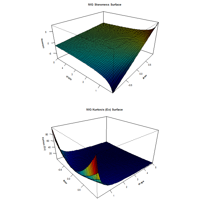
rugarch exports a set of functions for working with certain measures on the conditional distributions included in the package. Some of these functions have recently been re-written to take advantage of vectorization, whilst others re-written to take advantage of analytical representations (e.g. as regards to skewness and kurtosis measures for the sstd and jsu distributions). In the latest release, I’ve also included some functions which provide for a graphical visualization of the different distributions with regards to their higher moment features, and demonstrated below:
distplot('nig')
## Warning: skew lower bound below admissible region...adjusting to
## distribution lower bound.
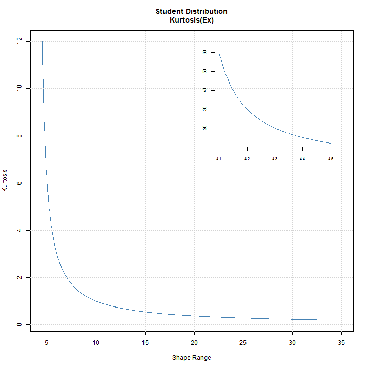
The distplot function, available for all skewed and/or shaped distributions provides a visual 3D representation of the interaction of the skew and shape parameters in determining the Skewness and Kurtosis. In cases where the distribution is only skewed or shaped, a simpler 2D plot is created as in the case of the std distribution:
distplot('std')
Another interesting plot is that of a distribution’s ‘authorized domain’, which shows the region of Skewness-Kurtosis for which a density exists. This is related to the Hamburger moment problem, and the maximum attainable Skewness (S) given kurtosis (K) ( see Widder (1946) ) . The skdomain function returns the values needed to visualize these relationships, and demonstrated below:
# plot the first one
XYnig = skdomain('nig', legend = FALSE)
XYsstd = skdomain('sstd', plot = FALSE)
XYhyp = skdomain('ghyp', plot = FALSE, lambda = 1)
XYjsu = skdomain('jsu', plot = FALSE)
# the values returned are the bottom half of the domain (which is
# symmetric)
lines(XYjsu$Kurtosis, XYjsu$Skewness, col = 3, lty = 2)
lines(XYjsu$Kurtosis, -XYjsu$Skewness, col = 3, lty = 2)
lines(XYsstd$Kurtosis, XYsstd$Skewness, col = 4, lty = 3)
lines(XYsstd$Kurtosis, -XYsstd$Skewness, col = 4, lty = 3)
lines(XYhyp$Kurtosis, XYhyp$Skewness, col = 5, lty = 4)
lines(XYhyp$Kurtosis, -XYhyp$Skewness, col = 5, lty = 4)
legend('topleft', c('MAX', 'NIG', 'JSU', 'SSTD', 'HYP'), col = c(2, 'steelblue', 3, 4, 5), lty = c(1, 1, 2, 3, 4), bty = 'n')
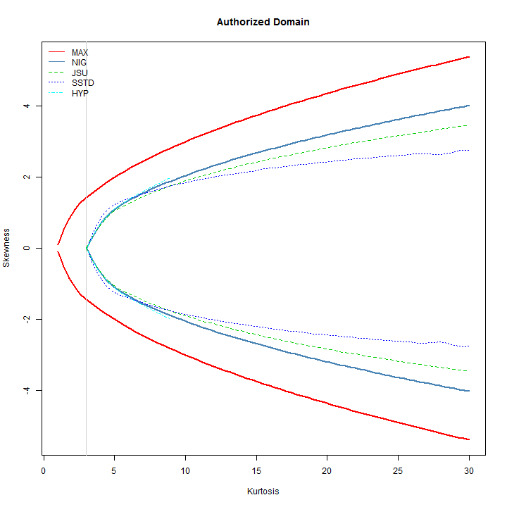
From the plot, it is clear that the skew-student has the widest possible combination of skewness and kurtosis for values of kurtosis less than ~6, whilst the NIG has the widest combination for values greater than ~8. It is interesting to note that the Hyperbolic distribution is not defined for values of kurtosis greater than ~9.
Model Reduction
The reduce function eliminates non-significant coefficients (subject to a pvalue cut-off argument) from a model by fixing them to zero (in rugarch this is equivalent to eliminating them) and re-estimating the model with the remaining parameters as the following example illustrates:
spec = ugarchspec(mean.model = list(armaOrder = c(4, 4)), variance.model = list(garchOrder = c(2, 2)))
fit = ugarchfit(spec, sp500ret[1:1000, ])
round(fit@fit$robust.matcoef, 4)
##         Estimate  Std. Error  t value Pr(>|t|)
## mu        0.0005      0.0004    1.250   0.2111
## ar1       0.2250      0.0164   13.677   0.0000
## ar2       1.6474      0.0175   94.046   0.0000
## ar3      -0.0661      0.0188   -3.517   0.0004
## ar4      -0.8323      0.0164  -50.636   0.0000
## ma1      -0.2328      0.0065  -35.825   0.0000
## ma2      -1.6836      0.0039 -430.423   0.0000
## ma3       0.0980      0.0098    9.953   0.0000
## ma4       0.8426      0.0075  112.333   0.0000
## omega     0.0000      0.0000    1.527   0.1267
## alpha1    0.2153      0.1265    1.702   0.0888
## alpha2    0.0000      0.0000    0.000   1.0000
## beta1     0.3107      0.1149    2.705   0.0068
## beta2     0.3954      0.0819    4.828   0.0000
##
# eliminate alpha2
fit = reduce(fit, pvalue = 0.1)
print(fit)
##
## *---------------------------------*
## *          GARCH Model Fit        *
## *---------------------------------*
##
## Conditional Variance Dynamics
## -----------------------------------
## GARCH Model  : sGARCH(2,2)
## Mean Model   : ARFIMA(4,0,4)
## Distribution : norm
##
## Optimal Parameters
## ------------------------------------
##         Estimate  Std. Error   t value Pr(>|t|)
## mu       0.00000          NA        NA       NA
## ar1      0.23153    0.006583   35.1698 0.000000
## ar2      1.63558    0.018294   89.4050 0.000000
## ar3     -0.07264    0.018277   -3.9743 0.000071
## ar4     -0.82110    0.014031  -58.5206 0.000000
## ma1     -0.23883    0.009659  -24.7253 0.000000
## ma2     -1.68338    0.005401 -311.6821 0.000000
## ma3      0.11434    0.017035    6.7121 0.000000
## ma4      0.83198    0.013140   63.3179 0.000000
## omega    0.00000          NA        NA       NA
## alpha1   0.14532    0.008997   16.1530 0.000000
## alpha2   0.00000          NA        NA       NA
## beta1    0.26406    0.086397    3.0564 0.002240
## beta2    0.58961    0.088875    6.6342 0.000000
##
## Robust Standard Errors:
##         Estimate  Std. Error  t value Pr(>|t|)
## mu       0.00000          NA       NA       NA
## ar1      0.23153    0.061687   3.7533 0.000175
## ar2      1.63558    0.093553  17.4829 0.000000
## ar3     -0.07264    0.024012  -3.0251 0.002485
## ar4     -0.82110    0.028395 -28.9168 0.000000
## ma1     -0.23883    0.037806  -6.3172 0.000000
## ma2     -1.68338    0.021478 -78.3771 0.000000
## ma3      0.11434    0.066989   1.7068 0.087851
## ma4      0.83198    0.052093  15.9711 0.000000
## omega    0.00000          NA       NA       NA
## alpha1   0.14532    0.057150   2.5428 0.010996
## alpha2   0.00000          NA       NA       NA
## beta1    0.26406    0.129725   2.0356 0.041793
## beta2    0.58961    0.103879   5.6759 0.000000
##
## LogLikelihood : 3091
## #####
References
Hansen, P. R., Lunde, A., & Nason, J. M. (2011). The model confidence set. Econometrica, 79(2), 453-497.
Widder, D. V. (1959). The Laplace Transform. 1946. Princeton University Press, Princeton, New Jersey. Supplementary Bibliography Is. McShane, EJ,“ A canonical form for antiderivatives,” Illinois Jour, of Math, 3, 334-351.
Is this code available now? I could really use it!
What do you mean “is this code available now?” ?
It’s been on CRAN for quite some time.
just noticed that. in the post you said the code had been moved to google code and I wasn’t sure what that meant.
The model reduction function shouldnt be used. The statisically valid way to do it is drop the higher pvalue regressor if it is above a cutoff and then refit the remaining regressors. Then repeat the process until all regressors are significant.
And how is this different from what the function allows you to do?
You choose the p-value for the cutoff, the coefficients above that are dropped and the model re-estimated. You can then repeat the process by re-submitting the object to the function.
Here’s the code to replicate the qq plot (which you can also call by type ‘plot(fit, which=9)’):
The main functionality can be found in the ‘rugarch:::.qqDist’ function.