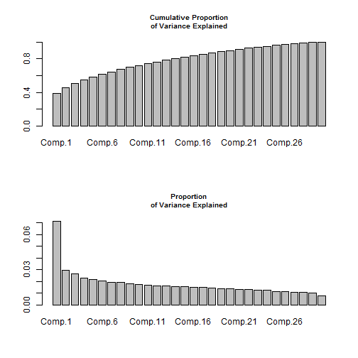
This demonstration illustrates the method described this blog post. I’m going to use the Dow30 constituents daily dataset and a benchmark based on equal weights. First we’ll investigate how many factors to estimate using PCA:
library(rmgarch)
library(parallel)
library(xts)
library(PerformanceAnalytics)
data(dji30ret)
# investigate PCA
pca = princomp(dji30ret)
par(mfrow = c(2, 1))
barplot(cumsum(summary(pca)$sdev^2)/sum(summary(pca)$sdev^2), main = 'Cumulative Proportion\nof Variance Explained', cex.main = 0.8)
barplot(summary(pca)$sdev, main = 'Proportion\nof Variance Explained', cex.main = 0.8)
We’ll use 10 for this application…and don’t ask my why. There are a number of paper which provide sophisticated methods for choosing the number of components using PCA and there is also random matrix theory for those so inclined which discusses the distribution of the eigenvalues and suitable cutoffs (see for example the futile.matrix package).
cl = makePSOCKcluster(10)
clusterEvalQ(cl, library(rmgarch))
X = as.xts(dji30ret)
spec = gogarchspec(mean.model = list(model = 'AR', lag = 1), variance.model = list(model = 'sGARCH',variance.targeting = TRUE), distribution = 'manig', ica = 'fastica')
mod = gogarchfit(spec, X, gfun = 'tanh', out.sample = 10, cluster = cl, maxiter1 = 1e+05, epsilon = 1e-07, rseed = 77, n.comp = 10)
Having estimated the model, the next step is to calculate the betas given the weights relative to the benchmark. Make sure to download the latest version of rmgarch from the teatime on r-forge which includes the necessary methods for doing so:
betaC = betacovar(mod, weights = rep(1/30, 30), asset = 1)
betaS = betacoskew(mod, weights = rep(1/30, 30), asset = 1, cluster = cl)
betaK = betacokurt(mod, weights = rep(1/30, 30), asset = 1, cluster = cl)
# also calculate the standard CAPM values from the PerformanceAnalytics
# package
bench = as.xts(apply(X, 1, 'mean'))
betaCK = cov(X[, 1], bench)/var(bench)
betaSK = BetaCoSkewness(X[, 1], bench)
betaKK = BetaCoKurtosis(X[, 1], bench)
par(mfrow = c(2, 2))
plot(betaC, type = 'l', main = '[CAPM] beta Covariance', cex.main = 0.9, auto.grid = FALSE,
    minor.ticks = FALSE, major.format = FALSE)
abline(h = betaCK, col = 2)
plot(betaS, type = 'l', main = '[CAPM] beta Coskewness', cex.main = 0.9, auto.grid = FALSE,
    minor.ticks = FALSE, major.format = FALSE)
abline(h = betaSK, col = 2)
plot(betaK, type = 'l', main = '[CAPM] beta Cokurtosis', cex.main = 0.9, auto.grid = FALSE,
    minor.ticks = FALSE, major.format = FALSE)
abline(h = betaKK, col = 2)
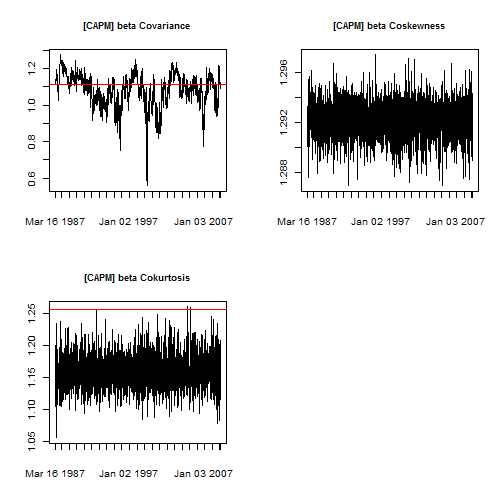
Obviously, absent of excess noise as a result of dimensionality reduction, the higher moment betas should not really vary too much since the GO-GARCH model does not explicitly model higher moment dynamics.
There are equivalent methods for working with objects of class goGARCHforecast and goGARCHfilter (though not as yet goGARCHsim). To illustrate, consider the forecasts based on rolling 1-ahead and unconditional n-ahead:
forc1 = gogarchforecast(mod, n.roll = 9, n.ahead = 1)
forc2 = gogarchforecast(mod, n.ahead = 10)
betaCf1 = betacovar(forc1, weights = rep(1/30, 30), asset = 1)
betaSf1 = betacoskew(forc1, weights = rep(1/30, 30), asset = 1)
betaKf1 = betacokurt(forc1, weights = rep(1/30, 30), asset = 1)
betaCf2 = betacovar(forc2, weights = rep(1/30, 30), asset = 1)
betaSf2 = betacoskew(forc2, weights = rep(1/30, 30), asset = 1)
betaKf2 = betacokurt(forc2, weights = rep(1/30, 30), asset = 1)
print(cbind(as.matrix(betaCf1), as.matrix(betaSf1), as.matrix(betaKf1)))
##            AA[T+1] AA[T+1] AA[T+1]
## 2009-01-20   1.068   1.371   1.081
## 2009-01-21   1.051   1.496   1.056
## 2009-01-22   1.045   1.522   1.051
## 2009-01-23   1.046   1.514   1.052
## 2009-01-26   1.043   1.519   1.049
## 2009-01-27   1.040   1.534   1.046
## 2009-01-28   1.038   1.592   1.043
## 2009-01-29   1.040   1.558   1.046
## 2009-01-30   1.049   1.481   1.055
## 2009-02-02   1.046   1.482   1.053
##
print(cbind(betaCf2, betaSf2, betaKf2))
##     AA[T0=2009-01-20] AA[T0=2009-01-20] AA[T0=2009-01-20]
## T+1             1.068             1.292             1.155
## T+2             1.068             1.292             1.159
## T+3             1.068             1.292             1.159
## T+4             1.068             1.292             1.157
## T+5             1.068             1.292             1.158
## T+6             1.068             1.292             1.159
## T+7             1.067             1.292             1.158
## T+8             1.067             1.292             1.159
## T+9             1.067             1.292             1.155
## T+10            1.067             1.292             1.155
Notice that the rolling forecast returns an xts object containing the T0 date as index for the T+1 forecast (see this blog post for more details), whilst the unconditional n-ahead forecast is a matrix with rownames the n.ahead period and column name the T0 date.

