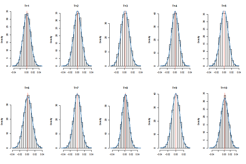
This short demo shows how to generate a simulated rolling forecast density. rugarch already has methods for generating analytic forecasts (ugarchforecast), rolling forecasts (ugarchroll) and bootstrap forecasts (ugarchboot).
library(rugarch)
data(sp500ret)
# use a default ARMA(1,1)-GARCH(1,1)-Normal specification
spec = ugarchspec()
N = nrow(sp500ret)
fit = ugarchfit(spec, sp500ret[1:1000, ])
# create a specification with fixed parameters:
specf = spec
setfixed(specf) < - as.list(coef(fit))
# we will create forecasts for T+1 to T+10 and for each simulated forecast
# use 5,000 points
fsim = matrix(NA, ncol = 10, nrow = 5000)
# we will also create the closed form forecast
afor = matrix(NA, ncol = 10, nrow = 2)
rownames(afor) = c('Mu', 'Sigma')
colnames(afor) = colnames(fsim) = paste('T+', 1:10, sep = '')
# T+1 we can use ugarchsim:
tmp = ugarchsim(fit, n.start = 0, startMethod = 'sample', n.sim = 1, m.sim = 5000)
fsim[, 1] = as.numeric(fitted(tmp))
tmp = ugarchforecast(fit, n.ahead = 1)
afor[, 1] = c(fitted(tmp), sigma(tmp))
# for T+(i>1):
for (i in 2:10) {
# filter the data upto time T+i-1 with the coefficients estimated from the
# model upto time T
filt = ugarchfilter(specf, data = sp500ret[1:(1000 + i - 1), ], n.old = 1000)
# use lagged values prior to the next forecast:
path = ugarchpath(specf, n.sim = 1, m.sim = 5000, presigma = tail(sigma(filt),
1), prereturns = sp500ret[(1000 + i - 1), ], preresiduals = tail(residuals(filt),
1))
# how do we know this is correct: check: path@path$seriesSim -
# path@path$residSim is the same with the analytical forecast of the
# series (below)
fsim[, i] = as.numeric(fitted(path))
tmp = ugarchforecast(specf, sp500ret[1:(1000 + i - 1), ], n.ahead = 1)
afor[, i] = c(fitted(tmp), sigma(tmp))
}
A visual check always helps:
# run some visual checks
par(mfrow = c(2, 5))
for (i in 1:10) {
hist(fsim[, i], freq = FALSE, col = 'WhiteSmoke', main = colnames(fsim)[i],
xlab = '')
abline(v = afor[1, i], col = 'tomato1')
curve(dnorm(x, mean = afor[1, i], sd = afor[2, i]), col = 'steelblue', lty = 1,
lwd = 2, add = TRUE)
}
Keep in mind that these simulated forecasts do not include parameter uncertainty…for that see the ugarchboot function. Finally, if you are wondering why this method of generating forecasts is important, note that it forms a key constituent to the 2-stage simulated multivariate density forecast in rmgarch which is used in stochastic programming and portfolio allocation.
