This example compares the in-sample goodness of fit of the DCC (MVN, MVT),and GO-GARCH(MVN, maNIG) model using the test of Hong and Li (2005). Because this is a univariate test, a set of randomly weighted vectors are used to create the weighted margins on which the Probability Integral Transform (PIT) is calculated for use with the test. This example is intended to highlight some of the methods and properties of these models as implemented in the rmgarch package. Note in particular how the weighted semi-analytic density of the GO-GARCH with maNIG distribution is calculated via the convolution (via FFT) method, the resulting object of which can then be passed to custom density (dfft), distribution (pfft), quantile (qfft) and sampling (rfft) functions. This application takes some time to calculate since every point in the insample weighted density has to be calculated for every weighting vector. In practice, it is usually the n-ahead forecast which is of interest on a fixed weighting vector which should be quite fast to calculate. In any case, the problem is separable and benefits from parallel computation.
library(rmgarch)
data(dji30retw)
library(parallel)
cl = makePSOCKcluster(10)
X = as.matrix(dji30retw)
uspec.n = multispec(replicate(30, ugarchspec(mean.model = list(armaOrder = c(1,0)))))
# DCC (MVN)
spec.dccn = dccspec(uspec.n, dccOrder = c(1, 1), distribution = 'mvnorm')
# DCC (MVT) with QML first stage
spec.dcct = dccspec(uspec.n, dccOrder = c(1, 1), distribution = 'mvt')
# GO-GARCH (MVN)
spec.ggn = gogarchspec(mean.model = list(model = 'AR', lag = 1), distribution.model = 'mvnorm', ica = 'fastica')
# GO-GARCH (maNIG)
spec.ggg = gogarchspec(mean.model = list(model = 'AR', lag = 1), distribution.model = 'manig', ica = 'fastica')
fit.1 = dccfit(spec.dccn, data = X, solver = 'solnp', cluster = cl, fit.control = list(eval.se = FALSE))
fit.2 = dccfit(spec.dcct, data = X, solver = 'solnp', cluster = cl, fit.control = list(eval.se = FALSE))
fit.3 = gogarchfit(spec.ggn, data = X, solver = 'hybrid', cluster = cl, gfun = 'tanh', maxiter1 = 40000, epsilon = 1e-08, rseed = 100)
fit.4 = gogarchfit(spec.ggg, data = X, solver = 'hybrid', cluster = cl, gfun = 'tanh', maxiter1 = 40000, epsilon = 1e-08, rseed = 100)
djisectors = c('Mat', 'Fin', 'Ind', 'Fin', 'Fin', 'Ind', 'Mat', 'Ind', 'Con', 'Ind', 'Con', 'Con', 'Tech', 'Tech', 'Tech', 'Hlth', 'Fin', 'Fin', 'Con', 'Con', 'Ind', 'Hlth', 'Tech', 'Hlth', 'Con', 'Tech', 'Tech', 'Tech', 'Con', 'Mat')
S = c('Mat', 'Fin', 'Ind', 'Con', 'Tech', 'Health')
S1 = which(djisectors == 'Mat')
S2 = which(djisectors == 'Fin')
S3 = which(djisectors == 'Ind')
S4 = which(djisectors == 'Con')
S5 = which(djisectors == 'Tech')
S6 = which(djisectors == 'Hlth')
# create the equal weights per sector
w1 = rep(1/length(S1), length(S1))
w2 = rep(1/length(S2), length(S2))
w3 = rep(1/length(S3), length(S3))
w4 = rep(1/length(S4), length(S4))
w5 = rep(1/length(S5), length(S5))
w6 = rep(1/length(S6), length(S6))
# Get the model based time varying covariance (arrays)
C1 = rcov(fit.1)
C2 = rcov(fit.2)
C3 = rcov(fit.3)
C4 = rcov(fit.4)
# create a quick function to generate the weighted sigma
indsig = function(S, idx, w) {
apply(S, 3, FUN = function(x) sqrt(w %*% x[idx, idx] %*% w))
}
C1.S = cbind(indsig(C1, S1, w1), indsig(C1, S2, w2), indsig(C1, S3, w3), indsig(C1, S4, w4), indsig(C1, S5, w5), indsig(C1, S4, w4))
C2.S = cbind(indsig(C2, S1, w1), indsig(C2, S2, w2), indsig(C2, S3, w3), indsig(C2, S4, w4), indsig(C2, S5, w5), indsig(C2, S4, w4))
C3.S = cbind(indsig(C3, S1, w1), indsig(C3, S2, w2), indsig(C3, S3, w3), indsig(C3, S4, w4), indsig(C3, S5, w5), indsig(C3, S4, w4))
C4.S = cbind(indsig(C4, S1, w1), indsig(C4, S2, w2), indsig(C4, S3, w3), indsig(C4, S4, w4), indsig(C4, S5, w5), indsig(C4, S4, w4))
# Extract the date and exclude first obs (AR-1 model)
Dt = as.Date(rownames(X))
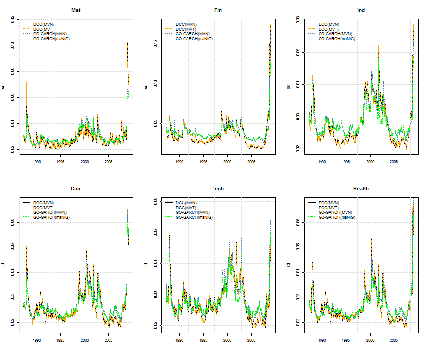
# plot equal weighted industry conditional volatility
par(mfrow = c(2, 3))
for (i in 1:6) {
plot(Dt, C1.S[, i], type = 'l', main = S[i], lty = 1, ylab = 'sd', xlab = ' ')
lines(Dt, C2.S[, i], col = 'orange', lty = 2)
lines(Dt, C3.S[, i], col = 'steelblue', lty = 3)
lines(Dt, C4.S[, i], col = 'green', lty = 4)
legend('topleft', c('DCC(MVN)', 'DCC(MVT)', 'GO-GARCH(MVN)', 'GO-GARCH(maNIG)'),
col = c('black', 'orange', 'steelblue', 'green'), lty = 1:4, bty = 'n')
grid()
}
# Mispecification Testing The testing is done on a randomly weighted
# set(in practise should be 1000+ randomly weighted portfolios).
w = matrix(rexp(30 * 100), 100, 30)
w = t(apply(w, 1, FUN = function(x) x/sum(x)))
HLp = array(NA, dim = c(100, 5, 4))
library(ff)
px = function(x, cf) {
    n = length(x)
    ans = rep(NA, n)
    for (i in 1:n) {
        pfun = pfft(cf, index = i)
        ans[i] = pfun(x[i])
    }
    return(ans)
}
for (i in 1:100) {
    # DCC distributions (being elliptical) have a nice 'wmargin' function
    wmarg1 = wmargin('mvnorm', weights = w[i, ], mean = fitted(fit.1), Sigma = C1)
    wmarg2 = wmargin('mvt', weights = w[i, ], mean = fitted(fit.2), Sigma = C2,
        shape = rshape(fit.2))
    wmarg3 = wmargin('mvnorm', weights = w[i, ], mean = fitted(fit.3), Sigma = C3)
    # this also works: wmarg3 = convolution(fit.3, weights = rep(1/30, 30))
    # GO-GARCH (non MVN) needs the convolution method maNIG weighted margins
    # estimated by FFT inversion of characteristic function
    wmarg4 = convolution(fit.4, weights = w[i, ], cluster = cl)
    p0 = as.numeric(X %*% w[i, ])
    p1 = pnorm(p0, wmarg1[, 1], wmarg1[, 2])
    p2 = pnorm(p0, wmarg2[, 1], wmarg2[, 2])
    p3 = pnorm(p0, wmarg3[, 1], wmarg3[, 2])
    p4 = px(p0, wmarg4)
    HLp[i, , 1] = HLTest(p1)$statistic
    HLp[i, , 2] = HLTest(p2)$statistic
    HLp[i, , 3] = HLTest(p3)$statistic
    HLp[i, , 4] = HLTest(p4)$statistic
}
# The HL test is one sided, normally distributed and nuisance parameter
# free.  Thus:
conf.level = 0.95
rejrate = qnorm(conf.level)
HLmedian = rbind(apply(HLp[, , 1], 2, FUN = function(x) median(x)), apply(HLp[,
    , 2], 2, FUN = function(x) median(x)), apply(HLp[, , 3], 2, FUN = function(x) median(x)),
    apply(HLp[, , 4], 2, FUN = function(x) median(x)))
HLrejections = rbind(apply(HLp[, , 1], 2, FUN = function(x) length(which(x >
    rejrate))/100), apply(HLp[, , 2], 2, FUN = function(x) length(which(x >
    rejrate))/100), apply(HLp[, , 3], 2, FUN = function(x) length(which(x >
    rejrate))/100), apply(HLp[, , 4], 2, FUN = function(x) length(which(x >
    rejrate))/100))
HLTable = matrix(NA, ncol = 5, nrow = 8)
HLTable[c(1, 3, 5, 7), ] = round(HLmedian, 3)
HLTable[c(2, 4, 6, 8), ] = round(HLrejections * 100, 0)
colnames(HLTable) = c('M(1,1)', 'M(2,2)', 'M(3,3)', 'M(4,4)', 'W')
rownames(HLTable) = c('DCC(MVN)', '%rej', 'DCC(MVT)', '%rej', 'GO-GARCH(MVN)',
    '%rej', 'GO-GARCH(maNIG)', '%rej')
print(HLTable)
##                 M(1,1) M(2,2) M(3,3) M(4,4)       W
## DCC(MVN)        -0.451  0.628  0.856  0.558   9.119
## %rej             2.000 26.000 35.000 20.000 100.000
## DCC(MVT)        -0.452  0.634  0.867  0.577   9.095
## %rej             2.000 26.000 35.000 20.000 100.000
## GO-GARCH(MVN)    0.082  0.922  0.920  0.359  18.132
## %rej            11.000 31.000 27.000 15.000 100.000
## GO-GARCH(maNIG)  0.027  0.895  0.855  0.272  12.570
## %rej            11.000 28.000 25.000 14.000 100.000
On the whole, none of the models fits the underlying dataset for this long period very well, as can be seen from the Portmanteau statistic (W) which is well outside the 5% significance level. The individual moment tests are not particularly indicative of the reason for this rejection since all models fall within the acceptance region. The GO-GARCH models appear to fare slightly better when it comes to the third and fourth moment conditional test (M(3,3) and M(4,4)), while the DCC models fare better in the first conditional moment test (M(1,1)) which may be the result of the AR dynamics being jointly estimated with GARCH in the first stage estimation of these models.