Despite its shortcomings, Value at Risk (VaR) is still the most widely used measure for measuring the risk of a portfolio, and the preferred measure in the Basel II Accord. In this demonstration, I backtest a group of indices using a GARCH-DCC(MVT) model and test the VaR obtained from randomly weighted portfolio margins using a number of relevant tests, based on functions in the rugarch and rmgarch packages. The use of randomly generated weights is in order to avoid any bias from testing a model with only equal weighted margins which is sometimes used. In practise, the weight vector is pre-determined, but for the backtesting, this approach appears a reasonable compromise for evaluating multivariate models using only univariate measures.
library(rmgarch)
library(quantmod)
# International Equity ETFs
Symbols = c('SPY', 'EWC', 'EWW', 'EWA', 'EWH', 'EWJ', 'EWS', 'EWG',
'EWQ', 'EWP', 'EWI', 'EWU', 'EWL', 'EWD')
m = length(Symbols)
Countries = c('USA', 'Canada', 'Mexico', 'Australia', 'Hong.Kong',
'Japan', 'Singapore', 'Germany', 'France', 'Spain', 'Italy', 'UK',
'Switzerland', 'Sweden')
getSymbols(Symbols, src = 'yahoo', from = '1990-01-01')
Y = Ad(SPY)
for (i in 2:m) Y = cbind(R, Ad(get(Symbols[i])))
Y = na.omit(Y)
R = ROC(Y, na.pad = FALSE)
It’s always a good idea to check the data visually for outliers or bad data:
par(mfrow = c(3, 5))
for (i in 1:m) hist(R[, i], breaks = 100, main = Countries[i])
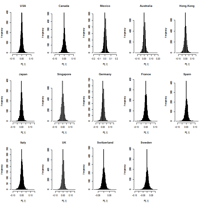
Not suprisingly, there is a large spike for the zeros in many countries and this is likely related to low volume when these ETFs where first introduced in the mid 1990s. I’ll exclude about 100 days from the start, since consecutive zeros in a dataset can seriously affect estimation (particularly a rolling backtest which does not use all the sample at once).
R = R[-c(1:100), ]
This is a ‘large’ scale backtest, so full use of parallel functionality is made, which is one of the features of the multivariate GARCH models included in the rmgarch package (the separability of the univariate from the multivariate dynamics).
A 2-stage QML DCC-(MVT) model (with first stage based ARMA(1,1)-gjrGARCH dynamics) is adopted, in the same spirit as in Bauwens and Laurent (2005). A separate post provides for an alternative approach using an iterated procedure for joint shape parameter estimation in the first stage conditional student density.
The model is estimated every 25 days (approx. 1 month), using all the data available up to that point, and the rolling 1-ahead forecast for the next 25 days is evaluated. The backtest procedure starts on 02-06-1999, thus providing an initial window for estimation of size 800, and ends on 10-19-2012 (the code adjusts to the last date available from the downloaded data.)
n = nrow(R)
roll = 25
start = 800
s = seq(start + roll, n, by = roll)
p = length(s)
out.sample = rep(roll, p)
if (s[p] < n) {
out.sample = c(out.sample, n - s[p])
s = c(s, n)
p = length(s)
}
500 sets of random weights (no shorts) are generated with full investment constraint (and for replicability the random seed is initialized to a predefined integer).
set.seed(111111)
w = matrix(rexp(14 * 500), 500, 14)
w = t(apply(w, 1, FUN = function(x) x/sum(x)))
w[500, ] = rep(1/m, m)
# create a required function for use later.
wsig = function(s, w) apply(w, 1, FUN = function(x) sqrt(x %*% s %*% x))
The backtest returns a list of length sum(out.sample)=3288 with elements the 25-rolling 1-ahead conditional forecasts of the mean and sigma weighted by the 500 random weight sets, and a vector of the shape parameter for each forecast window. While 2-stage DCC models offer the possibility of large scale parallel estimation because of the separation of the univariate and multivariate likelihoods, the calculation of the partitioned standard error (s.e.) matrix is quite slow (though this too can take advantage of parallel methods). For this application, s.e. are not calculated.
# set up the parallel estimation
library(parallel)
spec = multispec(replicate(m, ugarchspec(variance.model = list(model
= 'gjrGARCH'))))
mspec = dccspec(spec, distribution = 'mvt')
cl < - makePSOCKcluster(20)
clusterEvalQ(cl = cl, library(rmgarch))
clusterEvalQ(cl = cl, library(xts))
clusterExport(cl, varlist = c('R', 's', 'w', 'mspec', 'wsig', 'out.sample'),
envir = environment())
tic = Sys.time()
mod = clusterApply(cl = cl, 1:p, fun = function(i) {
fit = dccfit(mspec, R[1:s[i], ], out.sample = out.sample[i],
solver = 'solnp', fit.control = list(eval.se = FALSE))
f = dccforecast(fit, n.ahead = 1, n.roll = out.sample[i] - 1)
mu = t(apply(f@mforecast$mu, 3, FUN = function(x) x))
mu = apply(w, 1, FUN = function(x) mu %*% x)
# rcov(DCCforecast) is a list of size n.roll+1, with each
# element being an array of size m by m by n.ahead
sig = t(sapply(rcov(f), FUN = function(x) wsig(x[, , 1], w)))
shape = rep(as.numeric(rshape(fit)), out.sample[i])
dt = as.character(tail(time(R[1:s[i], ]), out.sample[i]))
ans = list(mu = mu, sig = sig, shape = shape, dates = dt)
return(ans)
})
toc = Sys.time()
stopCluster(cl)
The total time taken is about 3.62 mins, but with cloud based computing this could certainly be reduced, given that the functions themselves can take advantage of parallel estimation (not used here) to estimate the univariate models. Next, the forecasts are re-assembled and the VaR calculated, which because of the location and scaling invariant property of this distribution, is quite fast to evaluate.
mu = sig = shape = Dates = NULL
for (i in 1:length(mod)) {
mu = rbind(mu, mod[[i]]$mu)
sig = rbind(sig, mod[[i]]$sig)
shape = c(shape, mod[[i]]$shape)
Dates = c(Dates, mod[[i]]$dates)
}
# The realized weighted returns
realized = apply(w, 1, FUN = function(x) tail(R, sum(out.sample)) %*% x)
VaR01 = VaR05 = matrix(NA, ncol = 500, nrow = sum(out.sample))
for (i in 1:500) {
VaR01[, i] = mu[, i] + sig[, i] * qdist('std', 0.01, mu = 0, sigma = 1,
shape = shape)
VaR05[, i] = mu[, i] + sig[, i] * qdist('std', 0.05, mu = 0, sigma = 1,
shape = shape)
}
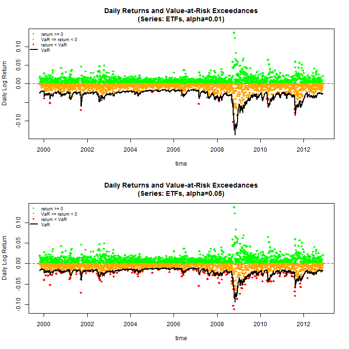
Before proceeding to the tests, do some plots to see some of the results (use the equal weighting margin=500)
par(mfrow = c(2, 1))
rugarch:::.VaRplot('ETFs', 0.01, realized[, 500], Dates, VaR01[, 500])
rugarch:::.VaRplot('ETFs', 0.05, realized[, 500], Dates, VaR05[, 500])
The test of VaR exceedances and VaR Duration are used, both of which are implemented and described in detail in the rugarch vignette and documentation. Once again, parallel functionality is used to evaluate these tests. For the exceedances test only the conditional coverage test is considered.
f = function(VaR, realized, p) {
tmp1 = VaRTest(p, realized, VaR)
tmp2 = VaRDurTest(p, realized, VaR)
Exceed = tmp1$actual.exceed
Excp = tmp1$cc.LRp
Excs = tmp1$cc.LRstat
Durb = tmp2$b
Durp = tmp2$LRp
return(c(Exceed = Exceed, Excp = Excp, Excs = Excs, Durb = Durb, Durp = Durp))
}
cl < - makeCluster(20)
clusterEvalQ(cl = cl, library(rugarch))
clusterExport(cl, varlist = c('VaR01', 'VaR05', 'f', 'realized'), envir = environment())
test1pct = clusterApply(cl = cl, 1:500, fun = function(i) f(VaR01[, i], realized[,
i], 0.01))
test5pct = clusterApply(cl = cl, 1:500, fun = function(i) f(VaR05[, i], realized[,
i], 0.05))
stopCluster(cl)
test1pct = t(sapply(test1pct, FUN = function(x) x))
test5pct = t(sapply(test5pct, FUN = function(x) x))
VaRresults = matrix(NA, ncol = 2, nrow = 5)
VaRDurresults = matrix(NA, ncol = 2, nrow = 3)
rownames(VaRDurresults) = c('Median_[b]', 'Median_pvalue', '%Rejections')
rownames(VaRresults) = c('Mean_Exceedances', 'E[Exceedances]', 'Median_stat',
'Median_pvalue', '%Rejections')
colnames(VaRDurresults) = colnames(VaRresults) = c('VaR[1%]', 'VaR[5%]')
VaRresults[1, ] = c(mean(test1pct[, 1]), mean(test5pct[, 1]))
VaRresults[2, ] = c(floor(sum(out.sample) * 0.01), floor(sum(out.sample) * 0.05))
VaRresults[3, ] = c(mean(test1pct[, 3]), median(test5pct[, 3]))
VaRresults[4, ] = c(mean(test1pct[, 2]), median(test5pct[, 2]))
VaRresults[5, ] = c(100 * length(which(test1pct[, 2] < 0.05))/nrow(test1pct),
100 * length(which(test5pct[, 2] < 0.05))/nrow(test5pct))
VaRDurresults[1, ] = c(median(test1pct[, 4]), median(test5pct[, 4]))
VaRDurresults[2, ] = c(median(test1pct[, 5]), median(test5pct[, 5]))
VaRDurresults[3, ] = c(100 * length(which(test1pct[, 5] < 0.05))/nrow(test1pct),
100 * length(which(test5pct[, 5] < 0.05))/nrow(test5pct))
The results summarized below tell an interesting story. The VaR Exceedances test indicates that at the 1% coverage the model used is unable to capture the extremes, with a rejection of the Null (H0: Correct Exceedances & Independent) in the region of 65% across all randomly weighted portfolios. However, when it comes to the 5% coverage the model does quite well with only a 13% rejection rate across all 500 portfolios. The VaR Duration test on the other hand, which measures the independence between exceedances (H0: Duration Between Exceedances have no memory (Weibull b=1 = Exponential)) has a rejection rate of less than 1% for both coverage rates indicating that the model used (ARMA-GARCH-DCC) is adequate for the modelling of the underlying dynamics, and the quantiles in particular. Nevertheless, exceedances for the 1% coverage are high and alternative dynamics may be called for, such as an Autoregressive Conditional Density model, a feasible multivariate example of which is presented in a recent paper by myself and colleagues The IFACD model.
print(VaRresults, digit = 2)
##                VaR[1%] VaR[5%]
## Exceedances     46.930     197
## E[Exceedances]  32.000     164
## Median_stat      6.666       0
## Median_pvalue    0.063       1
## %Rejections     65.400      13
##
##
print(VaRDurresults, digit = 2)
##               VaR[1%] VaR[5%]
## Median_[b]       0.98    1.00
## Median_pvalue    0.64    0.67
## %Rejections      0.20    0.20
References
Bauwens L and Laurent S (2005). “A new class of multivariate skew densities, with application to generalized autoregressive conditional
heteroscedasticity models.” Journal of Business and Economic Statistics, 23(3), pp. 346-354.